

Revolution in flow cytometry: using artificial intelligence for data processing and interpretation


Abstract
Flow cytometry (FC) represents a pivotal technique in the domain of biomedical research, facilitating the analysis of the physical and biochemical properties of cells. The advent of artificial intelligence (AI) algorithms has marked a significant turning point in the processing and interpretation of cytometric data, facilitating more precise and efficient analysis. The application of key AI algorithms, including clustering techniques (unsupervised learning), classification (supervised learning) and advanced deep learning methods, is becoming increasingly prevalent. Similarly, multivariate analysis and dimension reduction are also commonly attempted. The integration of advanced AI algorithms with FC methods contributes to a better understanding and interpretation of biological data, opening up new opportunities in research and clinical diagnostics. However, challenges remain in optimising the algorithms for the specificity of the cytometric data and ensuring their interpretability and reliability.
Citation
Bierzanowski S, Pietruczuk K. Revolution in flow cytometry: using artificial intelligence for data processing and interpretation. Eur J Transl Clin Med. 2025;8(1):83-96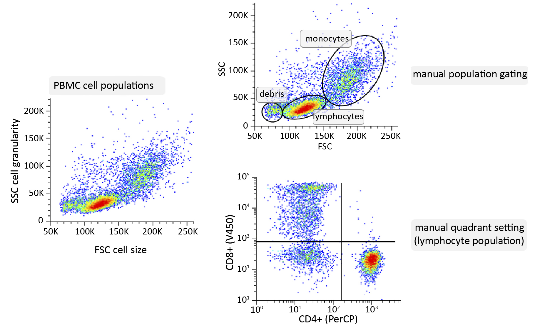


Introduction
Flow cytometry (FC) is a technique that enables rapid analysis of large numbers of cells in suspension by measuring the light scattered by the cells and fluorescence emitted by fluorochromes conjugated to antibodies [1-2]. The two main detectors are the forward scatter channel (FSC) which detects scattering along the laser beam, determining the size of particle and the side scatter channel (SSC) which measures scattering at 90°, thus assessing the granularity of the cells [3-4]. Other detectors measure the fluorescence produced by excitation of the fluorochrome with laser beam of the appropriate wavelength [3, 5].
FC is used in research and clinical laboratories for the assessment of cell surface antigen and intracellular antigen expression, enzyme activity gene expression and mRNA transcription [6]. This method permits the assessment of the cell cycle, mitochondria and cellular processes (e.g. apoptosis, autophagy, and cell ageing). It allows the quantification of biological substances in various body fluids, including serum and cerebrospinal fluid. FC allows not only the collection and analysis of data about cells, but also the sorting of cells based on the principle of deflecting flowing particles according to their electrical potential [6]. The degree of purity obtained is greater than 99%. This method is also employed to isolate rare cell populations, including cancer cells, fetal erythrocytes, and genetically modified cells [6-7]. The FC technique can be adapted for the detection, characterisation and enumeration of microorganisms in aqueous matrices, as well as somatic and bacterial cells in milk [8]. In medicine, FC is most widely used in haematology and oncology, specifically in cancer diagnosis, classification and monitoring treatment [7].
Despite the technological developments in FC, data analysis remains a key problem, requiring both standardisation and automation [9]. The aim of this article is to present the potential of AI algorithms in the analysis of cytometric data and the problems that still need to be solved to fully automate the process of analyzing this type of data.
Manual analysis of cytometric measurements
Manual gating still is the primary method for analysing the results. This step is essential for obtaining relevant information about the cells under study, whether the goal is to study the phenotype of a population or to identify the internal structures of cells [10]. In the case of the analysis of peripheral blood cells, such as lymphocytes, an FSC vs. SSC plot is initially constructed, which facilitates the distinction of the primary cell populations based on their size and granularity. Once the groups of cells of interest have been selected by setting up further gating, the expression of surface markers in fluorescence plots can be analysed. The manual gating process is complicated, time-consuming, subjectiveand requires advanced knowledge and experience [11-13].
Figure 1. Schematic of manual analysis of cytometric data using peripheral blood mononuclear cells (PBMC) sample as an example
Material and methods
The article is based on a review of the literature available in PubMed (biomedical research publications) and IEEE Xplore (broad access to technical literature in engineering and computer science). The analysis included articles on the application of machine learning algorithms to cytometric data analysis, including methods for mining and interpreting FC data. All included publications were selected for their relevance to the development of ML tools in this field.
Application of AI in cytometric data analysis
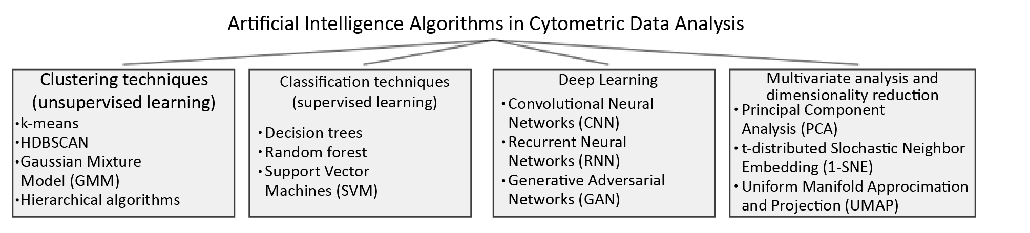
The use of artificial intelligence (AI) algorithms to automate the analysis of cytometric measurement data is becoming more common. This approach aims to reduce processing time and improve error resilience compared to manual methods. These algorithms mainly rely on clustering techniques, which involve dividing data based on specific criteria [14]. Clustering includes both classification (data is assigned to predefined classes) and clustering (natural groups in data without prior labels). Dimensionality reduction methods (e.g. principal component analysis, t-distributed stochastic neighbour embedding and uniform manifold approximation and projection) are also increasingly used.
Figure 2. Artifical Intelligence (AI) algorithms currently applicable to the analysis of cytometric measurements in analysis
Clustering techniques – unsupervised machine learning
Unsupervised learning, unlike supervised learning, operates on unlabeled data, identifying patterns and structures without pre-assigned categories.
k-means
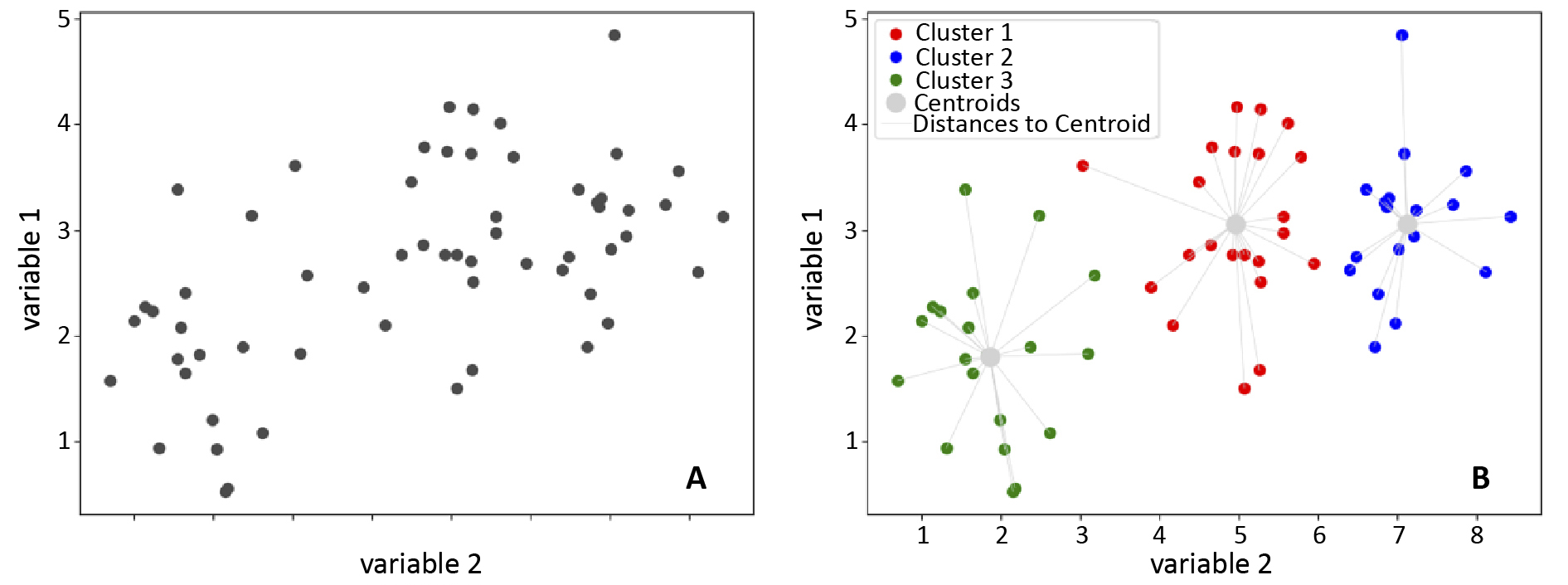
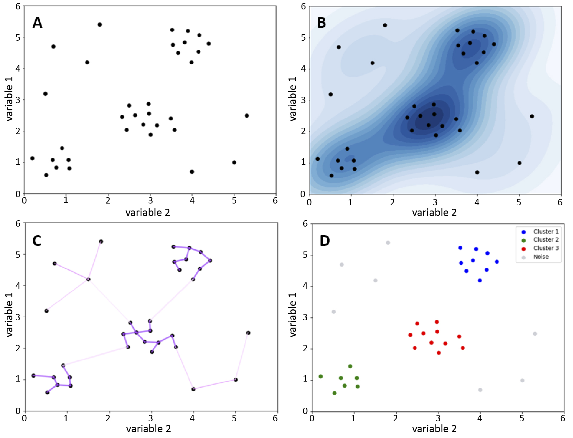
The first clustering algorithm used for analyzing cytometric data was k-means [15-16]. This iterative algorithm identifies data points with similar features around a central point called the ‘centroid’. Points closest to the centroid are grouped together, forming clusters. Distance is crucial in this algorithm and can be defined in various ways, but it is often the smallest sum of distances between the centroids and observations [17]. K-means involves several steps: selecting the number of clusters, initializing centroid positions, assigning each data point to the nearest centroid based on distance, recalculating centroids, and repeating these steps until the centroids’ positions stabilize or a stopping condition is met [15, 17].
Figure 3. Visualisation of the operation of k-means clustering algorithm
A – before the application of k-means; B – effect of the algorithm
K-means is a straightforward and effective clustering method, but it faces challenges like computational scalability, which can limit its use in analyzing cytometric data [18]. This algorithm requires substantial computation, with processing time increasing with the number of data points, clusters, and iterations, making it inefficient for large datasets like those from FC. Scalability can be improved by modifying the method to initialize centroids more efficiently or by using random data samples to update the centroids faster. Additionally, parallel computing is explored to further enhance scalability [19-20].
Another disadvantage of k-means is the need for the user to predefine the number of clusters [18]. Cytometric data are often characterised by a complex structure, which makes it difficult to determine the number of clusters, and choosing the wrong number of clusters can affect the biological interpretation of the results due to both under- and overestimation of their actual number [21]. When using the k-means algorithm, it is important to remember that it assumes the sphericity of the clusters and their separation [18]. These assumptions can be a disadvantage in the case of cytometric data obtained from peripheral blood cell measurements such as peripheral blood mononuclear cells (PBMC). This is because the cluster structure of these data is usually complex. PBMCs include different types of cell populations characterised by irregular distributions in the multidimensional feature space which may be caused, for example, by the fluorescence intensity of different surface markers [22]. At the same time, some cell populations have features that may lead to overlapping clusters causing the assumption of separation to fail.
A number of methods used in attempts to automate cytometric analysis have conceptual similarities to k-means or directly apply this algorithm. These methods include FlowClust, FlowMerge and FlowMeans [23-25]. Methods based on the k-means algorithm are often benchmarked and improved. The FlowMerge and flowClust algorithms were found useful in identifying cell populations in real clinical data from patients with chronic lymphocytic leukemia [23]. It was also pointed out that there were some difficulties in identifying clusters compared to other methods when evaluating their work with synthetic data [24].
Gaussian Mixture Model (GMM)
GMM is a probabilistic model that assumes data are generated from specific probability distributions [36]. It models data as a mixture of Gaussian components, each representing a cluster, estimating parameters like mean, variance and cluster weights to determine the likelihood of data points belonging to each cluster [37]. This makes GMM suitable for biomedical data analysis, including FC [38]. GMM is effective for clustering multimodal data with unknown cluster numbers, performing well with both continuous and discrete data, particularly when multiple peaks are present [39-40]. Cytometric data, such as PBMC phenotypes, often exhibit multimodality, making GMM ideal for identifying distinct cell populations, regardless of subtle differences [41-43]. The algorithm excels with continuous data and the Dirichlet Process Gaussian Mixture Model, an extension of GMM, handles unknown cluster numbers, automatically detecting clusters based on data structure [44-45].
HDBSCAN
Hierarchical Density-Based Spatial Clustering of Applications with Noise (HDBSCAN) is a density-based clustering algorithm [26-27] that groups closely located points and identifies outliers as noise. Unlike k-means, the HDBSCAN does not require a predetermined number of clusters, which makes it useful for analysing cytometric data when the number of subpopulations is unknown [27]. HDBSCAN adapts to different densities, identifies clusters of different shapes, but requires the definition of a minimum number of points to form a cluster and a distance measure [27]. This algorithm uses a hierarchical approach to clustering, assessing data membership based on their position in the cluster tree structure [28]. Points form a cluster if they are sufficiently densely packed, while points that do not meet the density criteria, i.e. without a sufficient number of neighbours within a certain radius, are treated as noise and remain unassigned [29-30].
HDBSCAN starts by calculating the distance of each point to its nearest neighbour, estimating the local density. Based on these distances, it creates a graph in which the points are vertices and the edges have weights corresponding to the distances of each other. This graph is used to create a minimum spanning tree, from which the edges with the lowest weights are iteratively removed, splitting the clusters [31]. Small clusters are labelled as noise and larger clusters are given new labels. Finally, the algorithm identifies the most stable clusters as the final result [30, 32]. Despite its efficiency, the HDBSCAN algorithm has a high computational complexity [28-30], making it slower than k-means [30].
Figure 4. The HDBSCAN clustering algorithm
A – scatter plot showing data points distributed across different feature space regions; B – darker colours indicate higher point concentration, suggesting potential clusters; lighter shades indicate lower density, possibly noise; C – graph where points are connected by edges weighted by their distances; D – HDBSCAN-identified clusters, with dense region points forming clusters and others labelled as noise (grey)
Automated analysis of cytometric data in oncology is crucial for faster and more objective patient monitoring. The combination of uniform manifold approximation and projection (UMAP) and HDBSCAN simultaneously reduces data dimensionality and identifies clusters in AML samples, effectively detecting blasts and improving monitoring of minimal residual disease. This approach is superior to traditional supervised methods, particularly with limited data and high variability of leukemic cells [33]. It was also suggested that the HDBSCAN algorithm is useful for the analysis of mitochondrial features by FC [34]. HDBSCAN is used to identify cell populations for cytometric analysis in some commercial programmes, although specific implementations vary depending on the specifics of the tool and analytical requirements [25, 35].
Classification techniques – supervised machine learning
Random forests
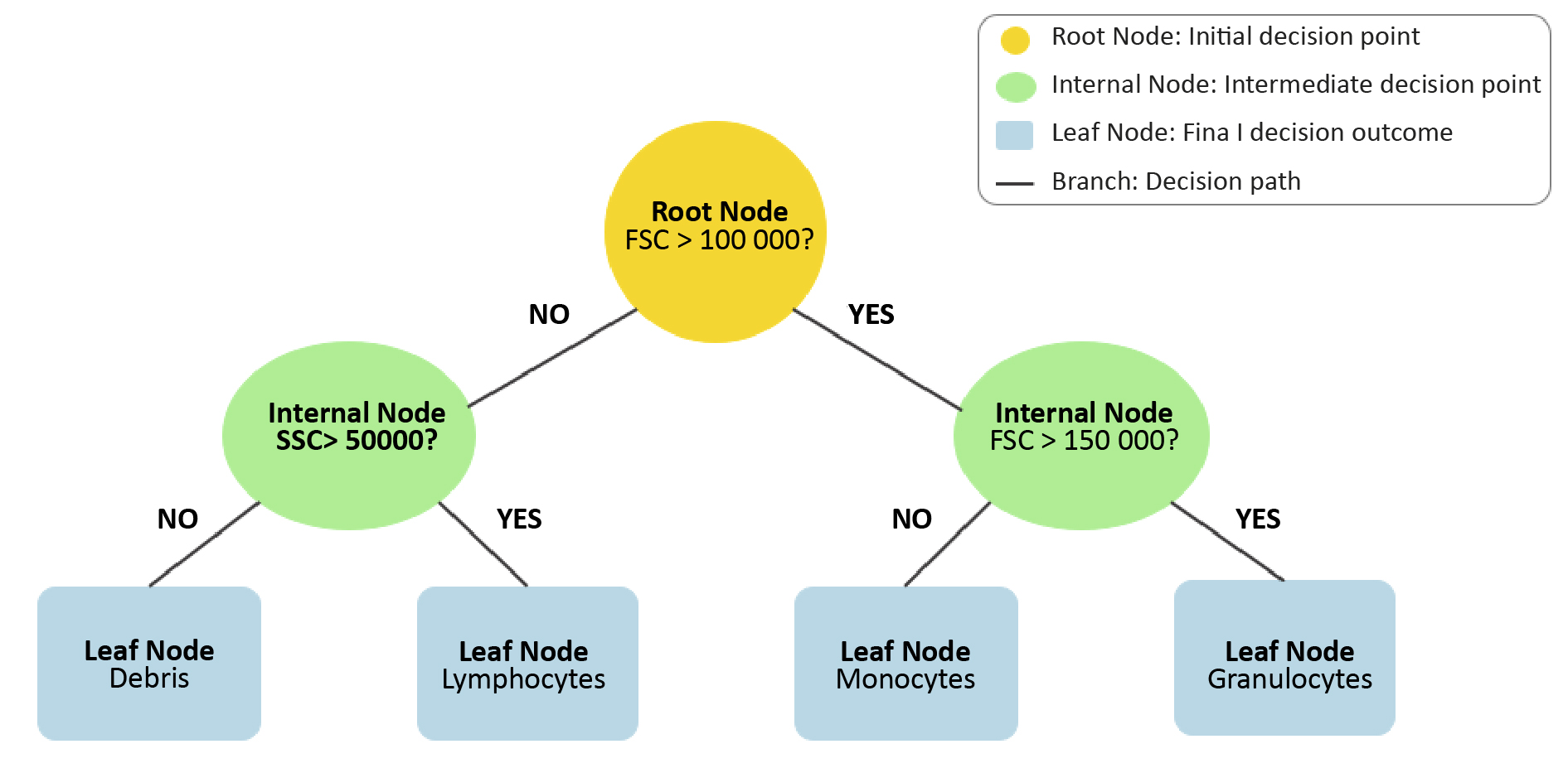
Random forest is one of the algorithms of supervised machine learning. The algorithm was developed by Breiman et al. [46]. It may be useful to conceptualise the structure of the proposed algorithm in terms of the organisation of a natural forest. A random forest is composed of individual trees, with each tree functioning as a classifier. These trees operate simultaneously to produce a collective classification output. This outcome is determined by a process of “voting” between the trees, with the result being the classification assigned to the input data.
The random forest algorithm is based on decision trees, which represent sets of decisions to solve problems. Decision trees consist of branches and nodes [47]. Key node types include: root (initial division), internal (specific choices), and leaf (final observations). Branches represent decision paths.
Figure 5. Visualization of a decision tree from Random Forests algorithm
The step-by-step classification process is shown through a series of decision nodes (yellow, green) and final classification outcomes at the leaf nodes (blue). The paths illustrate how data is split based on feature thresholds to reach the final decision.
There are several learning algorithms for decision trees, including: Id3, C4.5, CART, CHAID [48]. Decision trees are not complex structures, their implementation is relatively straightforward and does not require the appropriate scaling of features. They demonstrate high precision and accuracy in classification tasks, which is worth considering in analysis of FC data. On the other hand, they are not suitable for working on small datasets which can be a limitation in FC data analysis [49]. Presentation of the structure and functioning of decision trees is important in the context of the random forest algorithm because as mentioned earlier, random forests consist of multiple decision trees. The basic mechanism responsible for the generation of random forests is bagging (bootstrap aggregation), a method introduced by Breiman et al. [50]. It generates multiple predictor versions and later aggregates them. In random forests, bagging creates independent decision trees, each trained on unique bootstrap samples (random data samples with repetitions) [50]. The classification outcome is determined through a process known as majority voting. The technique of majority voting is a method of combining the predictions of results from multiple classifiers. Each decision tree “votes” for a class, and the class with the most votes becomes the final prediction [51-52]. This algorithm can be used as a classifier in cytometric data analysis.
Random forest, is an easy-to-implement machine learning algorithm, excels at detecting meaningful data patterns [53]. It can reveal subtle features often overlooked by traditional statistical methods. Those features are often crucial in the context of a medical diagnosis [54]. In one study, a random forest model was implemented to identify significant details within the acquired cytometric data, with the objective of increasing the accuracy of diagnosis. Researchers collected blood samples from 230 individuals, including those with myelodysplastic syndromes (MDS) and healthy controls. They then used FC to evaluate the cellular composition of these samples. A random forest model was utilized to analyse the collected cytometric data, facilitating the more accurate detection and classification of significant cellular patterns associated with MDS [54]. The ability of random forests to identify subtle relationships in complex, multi-parameter data has enabled researchers to diagnose the presence of myelodysplastic syndromes with greater accuracy. The model achieved 92% classification accuracy, a high and satisfactory result. The random forest algorithm is relatively resistant to overfitting, a situation in which the machine learning model provides good results based on the data on which it was trained, but is instead ineffective in analysing new, previously unseen data [55]. FC data can include many features (markers) for each cell, and the number of cells analysed is very large [56]. In such complex datasets, it is easy to have random patterns that can be misleading and lead to over-fitting, particularly when using simpler models such as single decision trees. Random forests are easy to interpret [53]. This is a major advantage in the context of cytometric data analysis. It helps to understand which features contribute to the classification of different cell populations. This makes it possible to identify biologically relevant markers [57], which is essential in the context of medical diagnostics and biomedical research. The model, which is simple to interpret, also makes it easier to verify results, which increases the reliability and precision of analyses.
While the random forest algorithm offers a number of advantages, it is not free from limitations that may affect its effective application in FC data analysis. A significant limitation of machine learning models is their high computational cost [58]. Cytometric data is frequently large and complex and multidimensional. As a result, training models based on this type of data can be costly and challenging from an economic perspective. Although random forests are resistant to over-fitting, in some cases they can be prone to this problem, especially when working with data containing a lot of noise. In the context of FC, we can interpret noisy data as data with measurement errors or issues caused by sample heterogeneity or biological variability [59-60], all of which can affect the generation and propagation of errors in the classification performed by the model.
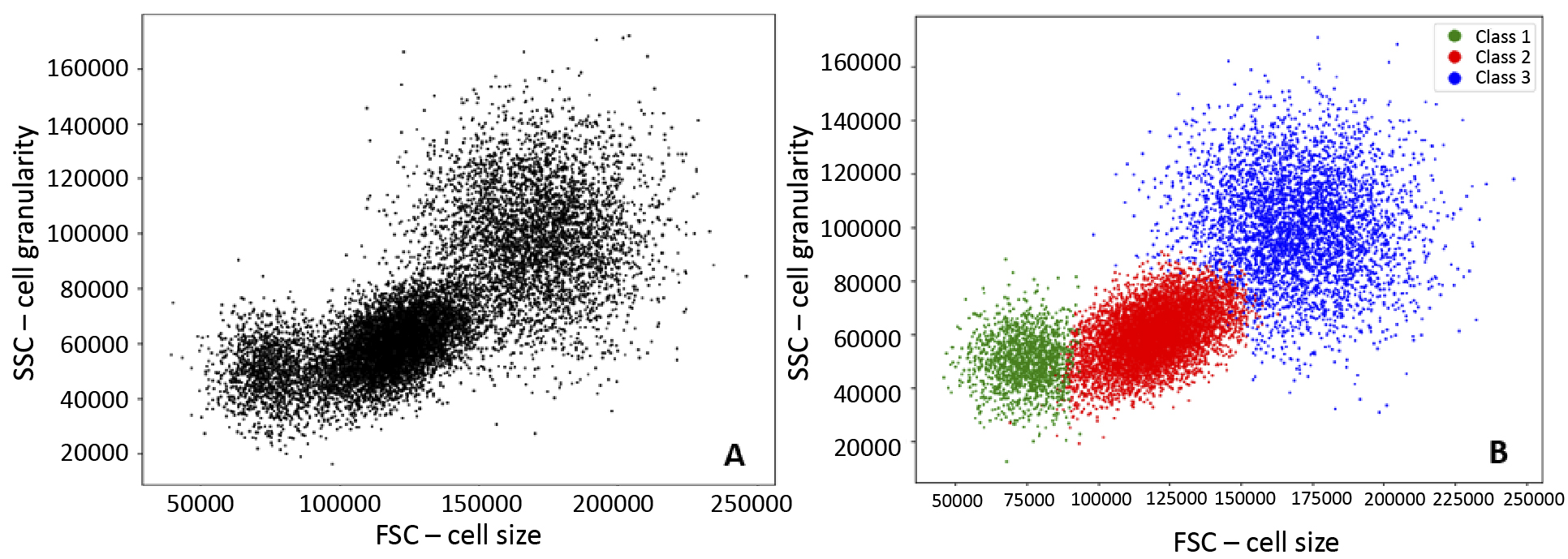
Figure 6. Visualisation of the implementation of Random Forests
A – before the application of Random Forests; B – effect of algorithm, classification into three groups
Support Vector Machines (SVM)
SVM was first introduced by Cortes and Vapnik et al. in 1995 [61]. The model was intended to be an effective alternative to the neural networks, which were still in development and presented certain technical challenges. SVM involves complex mathematical concepts including hyperplanes, margins, support vectors, kernels, and optimization. A hyperplane is a linear decision function that allows separation of data classes from each other. The prefix “hyper” indicates that this plane refers to multiple dimensions. For n dimensions, a hyperplane will take on (n–1) dimensions [61]. The margin is the distance between the hyperplane and the nearest data point [48]. Support vectors are data points that are located on a hyperplane. Optimization is the process of finding a hyperplane with as much margin as possible to best separate data points [62]. A kernel is a mathematical function that enables the transformation of data from a lower-dimensional space into a higher-dimensional space, allowing for the separation of the data [62]. In the context of FC data, an illustrative example would be the separation of cells in a PBMC graph with FSC and SSC parameters. In the two-dimensional space of the graph, it is not possible to linearly separate these cells. However, the kernel can be used to move the data points to a three-dimensional space, where it is possible to linearly separate them. The addition of an extra dimension allows for the creation of a hyperplane that can better represent the dataset.
SVM are particularly effective in classification tasks that require the detailed separation of data. One illustrative example is the use of a SVM as a classification tool for identifying circulating tumour cells (CTCs) in the bloodstream. In one study, blood samples were collected from 41 healthy individuals and 41 patients with colorectal cancer, and CTCs were counted on the basis of the results obtained from FC. An SVM classifier based on the number of CTCs was developed and achieved an 82.3% accuracy [63]. It has been demonstrated that the application of this cytometric data in the context of SVM learning can facilitate the effective differentiation between healthy and cancerous blood samples. The high performance of this model suggests its potential future use as a non-invasive cancer screening tool. SVM models are also suitable for identifying the presence of rare cells in peripheral blood. In one study, an SVM model was developed to identify rare cell types in FC data and it demonstrated an accuracy of 69%, compared to traditional manual classification. This tool could be used in the future for more precise analysis of FC data, particularly in the identification of rare cell types, which may be important in both disease diagnosis and therapy monitoring [64].
Despite their benefits, SVMs have limitations, particularly with data imbalance. FC datasets often contain underrepresented cell types, leading SVMs to create hyperplanes biased towards majority types, which may not be optimal for less abundant cell types [65]. Cytometric data are typically multidimensional and complex, necessitating careful kernel selection and parameter tuning to optimize model performance. This process, though time-consuming, is crucial to prevent over- or under-fitting [66-69]. Additionally, SVMs’ computational complexity in high-dimensional spaces can be a drawback, particularly in large cytometric datasets where rapid analysis is required [61, 70].
Deep learning
Although not new, deep learning has rapidly advanced due to increased computing power [71]. It is widely applied in medical fields, including immunology [72]. In simplified terms, neural networks learn through a two-stage process. First, the network receives a substantial amount of data, which it then uses to attempt to predict an outcome. Afterwards, it verifies the difference between the predicted outcome and the assumed outcome. This is an iterative process, in which the accuracy of the predictions is increased through the adjustment of weights. Each iteration results in a greater accuracy in the resulting predictions [73]. The actual learning process of neural networks is inherently complex, relying on several mathematical and statistical principles, which require deep understanding of linear algebra, calculus, probability and mathematical optimization. However it is possible to explain this process in much more simple terms by using one of the simplest models: a single-layer neural network.
To illustrate this, we can take the example of a manually curated FC dataset distinguishing healthy and cancerous cells. A single-layer neural network with an input layer and an output layer connected by randomly initialized weights is used. FC data, representing cell features, are entered, weighted, summed and passed through an activation function to capture patterns. The network predicts the cell’s type, and the error between the prediction and the true class is calculated. Using backpropagation, weights are adjusted iteratively to minimize the error [74-76].
In FC, deep learning enhances diagnostic efficiency by reducing analysis time and improving feature extraction [54]. Recent advancements have broadened its applications, even in challenging areas [77]. For example, a deep learning model effectively detected rare tumor cell clusters in breast cancer biopsies, though it showed lower sensitivity, indicating the need for larger datasets [78]. Deep learning models have achieved high efficiency in acute myeloid leukemia (AML) diagnosis, distinguishing AML from acute lymphoblastic leukemia with near-perfect accuracy [79]. Neural networks have proven effective in analysing multi-parameter flow cytometry data, aiding in leukemic classification [80-81]. Automation of pattern detection through neural networks significantly improves the precise classification of leukemic subtypes.
Deep learning in FC relies heavily on large training datasets, which may be challenging to obtain in smaller cytometric studies [78, 82]. Training complex neural networks also demands advanced hardware [71]. An additional drawback is the so-called “black box problem” which refers to the difficulty in explaining how a neural network makes specific decisions and generates the final outcome of its predictions [83]. In the context of cytometric data analysis, it is often unclear which specific cellular characteristics influenced the model to make certain diagnostic decisions. Simpler machine learning algorithms might sometimes offer more efficient solutions in this context.
Dimensionality reduction
Dimensionality reduction is an important group of machine learning methods, particularly in data analysis with many variables. It is the process of simplifying a dataset by reducing the number of variables, while retaining as much relevant information as possible [84]. This is the biggest advantage of the method, as a large number of variables often leads to problems with model over-fitting, often referred to as the ‘curse of dimensionality’ [85-86]. The second advantage is data compression and faster calculations [86]. The most commonly used methods for dimensionality reduction are principal component analysis (PCA), independent component analysis (ICA), t-Distributed Stochastic Neighbour Embedding (t-SNE) and the previously mentioned UMAP [87-89]. For cytometric data, t-SNE algorithm is often used in commercial software.
t-SNE is a non-linear, unsupervised technique mainly used for the exploration and visualisation of multivariate data [90]. It is a stochastic method, ordering ‘neighbours’ while preserving local data structures and using the Student’s t-distribution to model distances in low-dimensional space [91]. The algorithm allows separation of data that cannot be separated by a straight line, which is important for cytometric data.
It is a valuable tool in cell biology and immunological research, e.g. to profile cells of the immune system to understand their diversity, function and role in the immune response. The t-SNE algorithm has enabled the identification of subpopulations of normal and leukemic lyphocytec and the evaluation of their expression of immunosuppressive markers, clearly separating them from normal haematopoietic cells [92-93]. Combining t-SNE with unsupervised learning algorithms enables analysis of cytometric data to detect residual disease with high sensitivity [94]. The algorithm also supported the analysis of PBMC multicolour FC data, identifying rare subgroups of vaccine-induced T and B-cells [95].
Dimensionality reduction using t-SNE is effective in visualising immune cells and quantifying their frequencies, showing high agreement with conventional manual gating. However, it may not fully separate specific subsets of immune cells, leading to some discrepancies in the identification and quantification of these subpopulations, which is why the need to modify the algorithm in the analysis of cytometric data is highlighted, as standard parameter settings may lead to inaccurate or misleading cell maps [96-97]. The disadvantages of t-SNE are the high computational cost, difficult interpretation and need to set parameters that require tuning and experimentation.
Conclusions
Machine learning algorithms enable automated and precise data analysis, reducing errors due to subjectivity. However, we also face challenges. A key challenge is standardisation to ensure reproducibility and reliability. It is essential in laboratory diagnostics and biomedical sciences, as it enables comparison of results between laboratories and supports the introduction of modern techniques in routine diagnostics and clinical research. Without standardisation, it is difficult for these methods to be accepted in clinical practice. Other challenges include high computational costs, due to the fact that cytometric analyses involve multidimensional data of large size, requiring adequate memory resources and computing power. These costs can be reduced by optimising the performance of algorithms and using cloud-based solutions. As the computational complexity of the algorithms plays a key role here, a more practical selection of algorithms for specific cytometry applications also seems necessary.
Conflict of interest
None.
Funding
None.
References
| 1. |
Rieseberg M, Kasper C, Reardon KF, Scheper T. Flow cytometry in biotechnology. Appl Microbiol Biotechnol [Internet]. 2001;56(3):350–60. Available from: https://doi.org/10.1007/s002530100673.
|
| 2. |
El-Hajjar L, Ali Ahmad F, Nasr R. A Guide to Flow Cytometry: Components, Basic Principles, Experimental Design, and Cancer Research Applications. Curr Protoc [Internet]. 2023 Mar 1;3(3):e721. Available from: https://doi.org/10.1002/cpz1.721.
|
| 3. |
Sędek Ł, Sonsala A, Szczepański T, Mazur B. Techniczne aspekty cytometrii przepływowej [in Polish]. Diagnostyka Lab [Internet]. 2011;46(4):415–20. Available from: https://diagnostykalaboratoryjna.eu/article/59484/pl.
|
| 4. |
Skotny A, Pucińska J. Współczesna cystometria przepływowa [in Polish]. Acta Bio-Optica Inform Medica Inżynieria Biomed [Internet]. 2013;19(1):3–11. Available from: https://www.infona.pl/resource/bwmeta1.element.baztech-8a4c262e-3ba3-45d7-aba4-352e2eaa05a8?&locale=pl.
|
| 5. |
Sedek L, Mazur B. Przeciwciala monoklonalne i poliklonalne i ich zastosowanie w cytometrii przeplywowej [in Polish}. Postępy Biol Komórki Supl [Internet]. 2008;(24):17–34. Available from: https://agro.icm.edu.pl/agro/element/bwmeta1.element.agro-article-bc87278d-3186-4efe-ac85-f064303a1d3b.
|
| 6. |
Adan A, Alizada G, Kiraz Y, Baran Y, Nalbant A. Flow cytometry: basic principles and applications. Crit Rev Biotechnol [Internet]. 2017;37(2):163–76. Available from: https://doi.org/10.3109/07388551.2015.1128876.
|
| 7. |
Kaczmarek A, Mackiewicz A, Leporowska E, Osawa T. The role of flow cytometry in clinical diagnosis. Contemp Oncol Onkol [Internet]. 2002;6(6):366–73. Available from: https://www.termedia.pl/The-role-of-flow-cytometry-in-clinical-diagnosis,3,80,1,1.html.
|
| 8. |
S. GT, V. AP, A. VD. A Flow Cytometry Method for Rapid Detection and Enumeration of Total Bacteria in Milk. Appl Environ Microbiol [Internet]. 2000 Mar 1;66(3):1228–32. Available from: https://doi.org/10.1128/AEM.66.3.1228-1232.2000.
|
| 9. |
Brestoff JR, Frater JL. Contemporary Challenges in Clinical Flow Cytometry: Small Samples, Big Data, Little Time. J Appl Lab Med [Internet]. 2022 Jul 1;7(4):931–44. Available from: https://doi.org/10.1093/jalm/jfab176.
|
| 10. |
Bashashati A, Brinkman RR. A Survey of Flow Cytometry Data Analysis Methods. Adv Bioinformatics [Internet]. 2009 Dec 6;2009:1–19. Available from: https://www.hindawi.com/journals/abi/2009/584603/.
|
| 11. |
Montante S, Brinkman RR. Flow cytometry data analysis: Recent tools and algorithms. Int J Lab Hematol [Internet]. 2019 May 8;41(S1):56–62. Available from: https://onlinelibrary.wiley.com/doi/10.1111/ijlh.13016.
|
| 12. |
Tung JW, Heydari K, Tirouvanziam R, Sahaf B, Parks DR, Herzenberg LA, et al. Modern Flow Cytometry: A Practical Approach. Clin Lab Med [Internet]. 2007;27(3):453–68. Available from: https://www.sciencedirect.com/science/article/pii/S0272271207000467.
|
| 13. |
Caligola S, Giacobazzi L, Canè S, Vella A, Adamo A, Ugel S, et al. GateMeClass: Gate Mining and Classification of cytometry data. Elofsson A, editor. Bioinformatics [Internet]. 2024 May 2;40(5). Available from: https://academic.oup.com/bioinformatics/article/doi/10.1093/bioinformatics/btae322/7679648.
|
| 14. |
Jain AK, Murty MN, Flynn PJ. Data clustering. ACM Comput Surv [Internet]. 1999 Sep;31(3):264–323. Available from: https://dl.acm.org/doi/10.1145/331499.331504.
|
| 15. |
Aghaeepour N, Nikolic R, Hoos HH, Brinkman RR. Rapid cell population identification in flow cytometry data. Cytom Part A [Internet]. 2011 Jan 22;79A(1):6–13. Available from: https://onlinelibrary.wiley.com/doi/10.1002/cyto.a.21007.
|
| 16. |
Jain AK. Data clustering: 50 years beyond K-means. Pattern Recognit Lett [Internet]. 2010;31(8):651–66. Available from: https://www.sciencedirect.com/science/article/pii/S0167865509002323.
|
| 17. |
Hearty J. Advanced Machine Learning with Python [Internet]. Packt Publishing; 2016. Available from: https://books.google.pl/books?id=sc2qDQAAQBAJ.
|
| 18. |
Pelleg D. Extending K-means with efficient estimation of the number of clusters in ICML. In: Proceedings of the 17th international conference on machine learning. 2000. p. 277–81.
|
| 19. |
Tian X, Xu D, Guo L, Wu D. An Improved Bregman k-means++ Algorithm via Local Search BT - Computing and Combinatorics. In: Kim D, Uma RN, Cai Z, Lee DH, editors. Cham: Springer International Publishing; 2020. p. 532–41.
|
| 20. |
Hicks SC, Liu R, Ni Y, Purdom E, Risso D. mbkmeans: Fast clustering for single cell data using mini-batch k-means. Schneidman-Duhovny D, editor. PLOS Comput Biol [Internet]. 2021 Jan 26;17(1):e1008625. Available from: https://dx.plos.org/10.1371/journal.pcbi.1008625.
|
| 21. |
Piao Tan M, A. Floudas C. Determining the Optimal Number of Clusters. In: Encyclopedia of Optimization [Internet]. Boston, MA: Springer US; 2008. p. 687–94. Available from: https://link.springer.com/10.1007/978-0-387-74759-0_123.
|
| 22. |
Preglej T, Brinkmann M, Steiner G, Aletaha D, Göschl L, Bonelli M. Advanced immunophenotyping: A powerful tool for immune profiling, drug screening, and a personalized treatment approach. Front Immunol [Internet]. 2023 Mar 24;14. Available from: https://www.frontiersin.org/articles/10.3389/fimmu.2023.1096096/full.
|
| 23. |
Finak G, Bashashati A, Brinkman R, Gottardo R. Merging Mixture Components for Cell Population Identification in Flow Cytometry. Adv Bioinformatics [Internet]. 2009 Nov 12;2009:1–12. Available from: https://www.hindawi.com/journals/abi/2009/247646/.
|
| 24. |
Cheung M, Campbell JJ, Thomas RJ, Braybrook J, Petzing J. Assessment of Automated Flow Cytometry Data Analysis Tools within Cell and Gene Therapy Manufacturing. Int J Mol Sci [Internet]. 2022 Mar 17;23(6):3224. Available from: https://www.mdpi.com/1422-0067/23/6/3224.
|
| 25. |
Cheung M, Campbell JJ, Whitby L, Thomas RJ, Braybrook J, Petzing J. Current trends in flow cytometry automated data analysis software. Cytom Part A [Internet]. 2021 Oct 19;99(10):1007–21. Available from: https://onlinelibrary.wiley.com/doi/10.1002/cyto.a.24320.
|
| 26. |
Ram A, Jalal S, Jalal AS, Kumar M. A density based algorithm for discovering density varied clusters in large spatial databases. Int J Comput Appl [Internet]. 2010;3(6):1–4. Available from: https://www.researchgate.net/profile/Anant-Ram/publication/282334683_A_Density_based_Algorithm_for_Discovering_Density_Varied_Clusters_in_Large_Spatial_Databases/links/560d049d08aed543358d5e32/A-Density-based-Algorithm-for-Discovering-Density-Varied-Clust.
|
| 27. |
Campello RJGB, Moulavi D, Sander J. Density-Based Clustering Based on Hierarchical Density Estimates. In 2013. p. 160–72. Available from: http://link.springer.com/10.1007/978-3-642-37456-2_14.
|
| 28. |
Anibal J, Day AG, Bahadiroglu E, O’Neil L, Phan L, Peltekian A, et al. HAL-X: Scalable hierarchical clustering for rapid and tunable single-cell analysis. Faeder JR, editor. PLOS Comput Biol [Internet]. 2022 Oct 3;18(10):e1010349. Available from: https://dx.plos.org/10.1371/journal.pcbi.1010349.
|
| 29. |
Campello RJGB, Moulavi D, Zimek A, Sander J. Hierarchical Density Estimates for Data Clustering, Visualization, and Outlier Detection. ACM Trans Knowl Discov Data [Internet]. 2015 Jul 27;10(1):1–51. Available from: https://dl.acm.org/doi/10.1145/2733381.
|
| 30. |
Stewart G, Al-Khassaweneh M. An Implementation of the HDBSCAN* Clustering Algorithm. Appl Sci [Internet]. 2022 Feb 25;12(5):2405. Available from: https://www.mdpi.com/2076-3417/12/5/2405.
|
| 31. |
González-Alemán R, Platero-Rochart D, Rodríguez-Serradet A, Hernández-Rodríguez EW, Caballero J, Leclerc F, et al. MDSCAN: RMSD-based HDBSCAN clustering of long molecular dynamics. Martelli PL, editor. Bioinformatics [Internet]. 2022 Nov 30;38(23):5191–8. Available from: https://academic.oup.com/bioinformatics/article/38/23/5191/6751777.
|
| 32. |
Malzer C, Baum M. A Hybrid Approach To Hierarchical Density-based Cluster Selection. In: 2020 IEEE International Conference on Multisensor Fusion and Integration for Intelligent Systems (MFI) [Internet]. IEEE; 2020. p. 223–8. Available from: https://ieeexplore.ieee.org/document/9235263/.
|
| 33. |
Weijler L, Kowarsch F, Wödlinger M, Reiter M, Maurer-Granofszky M, Schumich A, et al. UMAP Based Anomaly Detection for Minimal Residual Disease Quantification within Acute Myeloid Leukemia. Cancers (Basel) [Internet]. 2022 Feb 11;14(4):898. Available from: https://www.mdpi.com/2072-6694/14/4/898.
|
| 34. |
Dhyani V, Chann AS, Giri L, Russell SM, Charnley M. A Pipeline for Dynamic Analysis of Mitochondrial Content in Developing T Cells: Bridging the Gap Between High-Throughput Flow Cytometry and Single-Cell Microscopy Analysis. In 2024. p. 167–87. Available from: https://link.springer.com/10.1007/978-1-0716-3834-7_12.
|
| 35. |
Ye X, Ho JWK. Ultrafast clustering of single-cell flow cytometry data using FlowGrid. BMC Syst Biol [Internet]. 2019 Apr 5;13(S2):35. Available from: https://bmcsystbiol.biomedcentral.com/articles/10.1186/s12918-019-0690-2.
|
| 36. |
Blekas K, Likas A, Galatsanos NP, Lagaris IE. A Spatially Constrained Mixture Model for Image Segmentation. IEEE Trans Neural Networks [Internet]. 2005 Mar;16(2):494–8. Available from: http://ieeexplore.ieee.org/document/1402510/.
|
| 37. |
Reynolds D. Gaussian Mixture Models. In: Encyclopedia of Biometrics [Internet]. Boston, MA: Springer US; 2009. p. 659–63. Available from: http://link.springer.com/10.1007/978-0-387-73003-5_196.
|
| 38. |
Pyne S, Hu X, Wang K, Rossin E, Lin T-I, Maier LM, et al. Automated high-dimensional flow cytometric data analysis. Proc Natl Acad Sci [Internet]. 2009 May 26;106(21):8519–24. Available from: https://pnas.org/doi/full/10.1073/pnas.0903028106.
|
| 39. |
McLachlan GJ, Ng SK, Peel D. On Clustering by Mixture Models. In: Schwaiger M, Opitz O, editors. Exploratory Data Analysis in Empirical Research Studies in Classification, Data Analysis, and Knowledge Organization [Internet]. Springer, Berlin, Heidelberg; 2003. p. 141–8. Available from: http://link.springer.com/10.1007/978-3-642-55721-7_16.
|
| 40. |
Dang UJ, Gallaugher MPB, Browne RP, McNicholas PD. Model-Based Clustering and Classification Using Mixtures of Multivariate Skewed Power Exponential Distributions. J Classif [Internet]. 2023;40(1):145–67. Available from: https://doi.org/10.1007/s00357-022-09427-7.
|
| 41. |
Zioulis N, Alexiadis D, Doumanoglou A, Louizis G, Apostolakis K, Zarpalas D, et al. 3D tele-immersion platform for interactive immersive experiences between remote users. In: 2016 IEEE International Conference on Image Processing (ICIP) [Internet]. IEEE; 2016. p. 365–9. Available from: http://ieeexplore.ieee.org/document/7532380/.
|
| 42. |
Sun P, Lyu X, Li X, Wang B, Yi X, Tang Z. Understanding Markush Structures in Chemistry Documents With Deep Learning. In: 2018 IEEE International Conference on Bioinformatics and Biomedicine (BIBM) [Internet]. IEEE; 2018. p. 1126–9. Available from: https://ieeexplore.ieee.org/document/8621264/.
|
| 43. |
Rajwa B, Wallace PK, Griffiths EA, Dundar M. Automated Assessment of Disease Progression in Acute Myeloid Leukemia by Probabilistic Analysis of Flow Cytometry Data. IEEE Trans Biomed Eng. 2017;64(5):1089–98.
|
| 44. |
Reiter M, Rota P, Kleber F, Diem M, Groeneveld-Krentz S, Dworzak M. Clustering of cell populations in flow cytometry data using a combination of Gaussian mixtures. Pattern Recognit [Internet]. 2016 Dec;60:1029–40. Available from: https://linkinghub.elsevier.com/retrieve/pii/S0031320316300371.
|
| 45. |
Yerebakan HZ, Rajwa B, Dundar M. The infinite mixture of infinite Gaussian mixtures. In: Advances in neural information processing systems. 2014.
|
| 46. |
Breiman L. Random Forests. Mach Learn [Internet]. 2001;45(1):5–32. Available from: https://doi.org/10.1023/A:1010933404324.
|
| 47. |
Song Y-Y, Lu Y. Decision tree methods: applications for classification and prediction. Shanghai Arch psychiatry [Internet]. 2015 Apr 25;27(2):130–5. Available from: http://www.ncbi.nlm.nih.gov/pubmed/26120265.
|
| 48. |
Burges CJC. A Tutorial on Support Vector Machines for Pattern Recognition. Data Min Knowl Discov [Internet]. 1998;2(2):121–67. Available from: https://doi.org/10.1023/A:1009715923555.
|
| 49. |
Khare S, Gourisaria MK, Harshvardhan G, Joardar S, Singh V. Real Estate Cost Estimation Through Data Mining Techniques. IOP Conf Ser Mater Sci Eng [Internet]. 2021 Mar 1;1099(1):012053. Available from: https://iopscience.iop.org/article/10.1088/1757-899X/1099/1/012053.
|
| 50. |
Breiman L. Bagging predictors. Mach Learn [Internet]. 1996;24(2):123–40. Available from: https://doi.org/10.1007/BF00058655.
|
| 51. |
Zamahsyari, Nurwidyantoro A. Sentiment analysis of economic news in Bahasa Indonesia using majority vote classifier. In: 2016 International Conference on Data and Software Engineering (ICoDSE). 2016. p. 1–6.
|
| 52. |
Daho MEH, Settouti N, Lazouni MEA, Chikh MEA. Weighted vote for trees aggregation in Random Forest. In: 2014 International Conference on Multimedia Computing and Systems (ICMCS). 2014. p. 438–43.
|
| 53. |
Salam MA, Taher A, Samy M, Mohamed K. The Effect of Different Dimensionality Reduction Techniques on Machine Learning Overfitting Problem. Int J Adv Comput Sci Appl [Internet]. 2021;12(4). Available from: http://thesai.org/Publications/ViewPaper?Volume=12&Issue=4&Code=IJACSA&SerialNo=80.
|
| 54. |
Palit S, Heuser C, de Almeida GP, Theis FJ, Zielinski CE. Meeting the Challenges of High-Dimensional Single-Cell Data Analysis in Immunology. Front Immunol [Internet]. 2019 Jul 3;10. Available from: https://www.frontiersin.org/article/10.3389/fimmu.2019.01515/full.
|
| 55. |
Duetz C, Van Gassen S, Westers TM, van Spronsen MF, Bachas C, Saeys Y, et al. Computational flow cytometry as a diagnostic tool in suspected‐myelodysplastic syndromes. Cytom Part A [Internet]. 2021 Aug 12;99(8):814–24. Available from: https://onlinelibrary.wiley.com/doi/10.1002/cyto.a.24360.
|
| 56. |
Dietterich T. Overfitting and undercomputing in machine learning. ACM Comput Surv [Internet]. 1995 Sep;27(3):326–7. Available from: https://dl.acm.org/doi/10.1145/212094.212114.
|
| 57. |
Boin F, Giardino Torchia ML, Borrello I, Noonan KA, Neil M, Soloski MJ, et al. Flow cytometric discrimination of seven lineage markers by using two fluorochromes. Björkström NK, editor. PLoS One [Internet]. 2017 Nov 30;12(11):e0188916. Available from: https://dx.plos.org/10.1371/journal.pone.0188916.
|
| 58. |
Bolón-Canedo V, Morán-Fernández L, Cancela B, Alonso-Betanzos A. A review of green artificial intelligence: Towards a more sustainable future. Neurocomputing [Internet]. 2024;599:128096. Available from: https://www.sciencedirect.com/science/article/pii/S0925231224008671.
|
| 59. |
Mazza EMC, Brummelman J, Alvisi G, Roberto A, De Paoli F, Zanon V, et al. Background fluorescence and spreading error are major contributors of variability in high‐dimensional flow cytometry data visualization by t‐distributed stochastic neighboring embedding. Cytom Part A [Internet]. 2018 Aug 14;93(8):785–92. Available from: https://onlinelibrary.wiley.com/doi/10.1002/cyto.a.23566.
|
| 60. |
Browning AP, Ansari N, Drovandi C, Johnston APR, Simpson MJ, Jenner AL. Identifying cell-to-cell variability in internalization using flow cytometry. J R Soc Interface [Internet]. 2022 May 25;19(190). Available from: https://royalsocietypublishing.org/doi/10.1098/rsif.2022.0019.
|
| 61. |
Awad M, Khanna R. Support Vector Machines for Classification. In: Efficient Learning Machines [Internet]. Berkeley, CA: Apress; 2015. p. 39–66. Available from: http://link.springer.com/10.1007/978-1-4302-5990-9_3.
|
| 62. |
Noble WS. What is a support vector machine? Nat Biotechnol [Internet]. 2006 Dec;24(12):1565–7. Available from: https://www.nature.com/articles/nbt1206-1565.
|
| 63. |
Hatzidaki E, Iliopoulos A, Papasotiriou I. A Novel Method for Colorectal Cancer Screening Based on Circulating Tumor Cells and Machine Learning. Entropy (Basel) [Internet]. 2021 Sep 25;23(10). Available from: http://www.ncbi.nlm.nih.gov/pubmed/34681972.
|
| 64. |
Special Issue Title Page. Cytom Part A [Internet]. 2015 Jun 28;87(6). Available from: https://onlinelibrary.wiley.com/doi/10.1002/cyto.a.22695.
|
| 65. |
Mair F, Hartmann FJ, Mrdjen D, Tosevski V, Krieg C, Becher B. The end of gating? An introduction to automated analysis of high dimensional cytometry data. Eur J Immunol [Internet]. 2016 Jan 30;46(1):34–43. Available from: https://onlinelibrary.wiley.com/doi/10.1002/eji.201545774.
|
| 66. |
Núñez H, Gonzalez-Abril L, Angulo C. Improving SVM Classification on Imbalanced Datasets by Introducing a New Bias. J Classif [Internet]. 2017 Oct 14;34(3):427–43. Available from: http://link.springer.com/10.1007/s00357-017-9242-x.
|
| 67. |
Huang Y, Zhao H, Shao M, Zhou L, Li X, Wei G, et al. Predictive value of next-generation sequencing-based minimal residual disease after CAR-T cell therapy. Bone Marrow Transplant [Internet]. 2022 Aug 1;57(8):1350–3. Available from: https://www.nature.com/articles/s41409-022-01699-2.
|
| 68. |
Chakraborty R, Al Hadidi S, Scheffer Cliff ER, Mohyuddin GR. Is aggressive treatment of smoldering myeloma the path to curing myeloma? Blood Adv [Internet]. 2023 Aug 8;7(15):3932–5. Available from: https://ashpublications.org/bloodadvances/article/7/15/3932/495857/Is-aggressive-treatment-of-smoldering-myeloma-the.
|
| 69. |
Biehl M, Bunte K, Schneider P. Analysis of Flow Cytometry Data by Matrix Relevance Learning Vector Quantization. Ma’ayan A, editor. PLoS One [Internet]. 2013 Mar 18;8(3):e59401. Available from: https://dx.plos.org/10.1371/journal.pone.0059401.
|
| 70. |
Aghaeepour N, Finak G, Hoos H, Mosmann TR, Brinkman R, Gottardo R, et al. Critical assessment of automated flow cytometry data analysis techniques. Nat Methods [Internet]. 2013 Mar 10;10(3):228–38. Available from: https://www.nature.com/articles/nmeth.2365.
|
| 71. |
Thompson NC, Greenewald K, Lee K, Manso GF. The computational limits of deep learning. arXiv Prepr arXiv200705558 [Internet]. 2020;10. Available from: http://arxiv.org/abs/2007.05558.
|
| 72. |
Matsuda A, Imada K, Obara N, Iida H, Yamazaki H, Tomiyama Y, et al. Dysmegakaryopoiesis and Transient Mild Increase in Bone Marrow Blasts in Patients With Aplastic Anemia Treated With Eltrombopag May Be Signs of Hematologic Improvement and Not Portend Clonal Evolution. Am J Clin Pathol [Internet]. 2022 Nov 3;158(5):604–15. Available from: https://academic.oup.com/ajcp/article/158/5/604/6677142.
|
| 73. |
Grossi E, Buscema M. Introduction to artificial neural networks. Eur J Gastroenterol Hepatol [Internet]. 2007 Dec;19(12):1046–54. Available from: http://journals.lww.com/00042737-200712000-00005.
|
| 74. |
Feng Y, Cheng Z, Chai H, He W, Huang L, Wang W. Neural network-enhanced real-time impedance flow cytometry for single-cell intrinsic characterization. Lab Chip [Internet]. 2022;22(2):240–9. Available from: https://xlink.rsc.org/?DOI=D1LC00755F.
|
| 75. |
Fisch L, Heming M, Schulte-Mecklenbeck A, Gross CC, Zumdick S, Barkhau C, et al. GateNet: A novel neural network architecture for automated flow cytometry gating. Comput Biol Med [Internet]. 2024 Sep;179:108820. Available from: https://linkinghub.elsevier.com/retrieve/pii/S0010482524009053.
|
| 76. |
Bini L, Mojarrad FN, Liarou M, Matthes T, Marchand-Maillet S. FlowCyt: A Comparative Study of Deep Learning Approaches for Multi-Class Classification in Flow Cytometry Benchmarking. arXiv Prepr arXiv240300024 [Internet]. 2024; Available from: https://doi.org/10.48550/arXiv.2403.00024.
|
| 77. |
Sun C, Shrivastava A, Singh S, Gupta A. Revisiting unreasonable effectiveness of data in deep learning era. In: Proceedings of the IEEE international conference on computer vision [Internet]. 2017. p. 843–52. Available from: https://openaccess.thecvf.com/content_iccv_2017/html/Sun_Revisiting_Unreasonable_Effectiveness_ICCV_2017_paper.html.
|
| 78. |
Vora N, Shekar P, Esmail M, Patra A, Georgakoudi I. Deep Learning-Enabled, Detection of Rare Circulating Tumor Cell Clusters in Whole Blood Using Label-free, Flow Cytometry [Internet]. 2023. Available from: http://biorxiv.org/lookup/doi/10.1101/2023.08.01.551485.
|
| 79. |
Lewis JE, Cooper LAD, Jaye DL, Pozdnyakova O. Automated Deep Learning-Based Diagnosis and Molecular Characterization of Acute Myeloid Leukemia Using Flow Cytometry. Mod Pathol [Internet]. 2024;37(1):100373. Available from: https://www.sciencedirect.com/science/article/pii/S0893395223002788.
|
| 80. |
Kothari R, Cualing H, Balachander T. Neural network analysis of flow cytometry immunophenotype data. IEEE Trans Biomed Eng [Internet]. 1996;43(8):803–10. Available from: http://ieeexplore.ieee.org/document/508551/.
|
| 81. |
Magallon RE, Harmacek LD, Arger NK, Grewal P, Powers L, Werner BR, et al. Standardization of flow cytometry and cell sorting to enable a transcriptomic analysis in a multi-site sarcoidosis study. Chitta S, editor. PLoS One [Internet]. 2023 Mar 9;18(3):e0281210. Available from: https://dx.plos.org/10.1371/journal.pone.0281210.
|
| 82. |
Sarker IH. Deep Learning: A Comprehensive Overview on Techniques, Taxonomy, Applications and Research Directions. SN Comput Sci [Internet]. 2021 Nov 18;2(6):420. Available from: https://link.springer.com/10.1007/s42979-021-00815-1.
|
| 83. |
Hassija V, Chamola V, Mahapatra A, Singal A, Goel D, Huang K, et al. Interpreting Black-Box Models: A Review on Explainable Artificial Intelligence. Cognit Comput [Internet]. 2024 Jan 24;16(1):45–74. Available from: https://link.springer.com/10.1007/s12559-023-10179-8.
|
| 84. |
Goldenberg A. A Survey of Statistical Network Models. Found Trends® Mach Learn [Internet]. 2009;2(2):129–233. Available from: http://www.nowpublishers.com/article/Details/MAL-005.
|
| 85. |
Verleysen M, François D. The Curse of Dimensionality in Data Mining and Time Series Prediction. In: Cabestany J, Prieto A, Sandoval F, editors. Computational Intelligence and Bioinspired Systems [Internet]. Berlin, Heidelberg; 2005. p. 758–70. Available from: http://link.springer.com/10.1007/11494669_93.
|
| 86. |
Hastie T, Tibshirani R, Friedman J. High-Dimensional Problems: p N. In 2009. p. 649–98. Available from: http://link.springer.com/10.1007/978-0-387-84858-7_18.
|
| 87. |
Jolliffe IT. Principal component analysis for special types of data [Internet]. New York: Springer; 2002. Available from: https://link.springer.com/content/pdf/10.1007/0-387-22440-8_13.pdf.
|
| 88. |
Hyvärinen A, Hurri J, Hoyer PO. Independent Component Analysis. In Springer; 2009. p. 151–75. Available from: http://link.springer.com/10.1007/978-1-84882-491-1_7.
|
| 89. |
McInnes L, Healy J, Saul N, Großberger L. UMAP: Uniform Manifold Approximation and Projection. J Open Source Softw [Internet]. 2018 Sep 2;3(29):861. Available from: http://joss.theoj.org/papers/10.21105/joss.00861.
|
| 90. |
Van der Maaten L, Hinton G. Visualizing data using t-SNE. J Mach Learn Res [Internet]. 2008;9(11). Available from: http://www.jmlr.org/papers/volume9/vandermaaten08a/vandermaaten08a.pdf.
|
| 91. |
Hinton GE, Salakhutdinov RR. Reducing the Dimensionality of Data with Neural Networks. Science (80- ) [Internet]. 2006 Jul 28;313(5786):504–7. Available from: https://www.science.org/doi/10.1126/science.1127647.
|
| 92. |
Retraction: Regulation of Tumor Cell Sensitivity to TRAIL-Induced Apoptosis by the Metastatic Suppressor Raf Kinase Inhibitor Protein via Yin Yang 1 Inhibition and Death Receptor 5 Up-Regulation. J Immunol [Internet]. 2016 Dec 15;197(12):4859–4859. Available from: https://journals.aai.org/jimmunol/article/197/12/4859/109147/Retraction-Regulation-of-Tumor-Cell-Sensitivity-to.
|
| 93. |
Nollmann C, Moskorz W, Wimmenauer C, Jäger PS, Cadeddu RP, Timm J, et al. Characterization of CD34+ Cells from Patients with Acute Myeloid Leukemia (AML) and Myelodysplastic Syndromes (MDS) Using a t-Distributed Stochastic Neighbor Embedding (t-SNE) Protocol. Cancers (Basel) [Internet]. 2024 Mar 28;16(7):1320. Available from: https://www.mdpi.com/2072-6694/16/7/1320.
|
| 94. |
Matthes T. Phenotypic Analysis of Hematopoietic Stem and Progenitor Cell Populations in Acute Myeloid Leukemia Based on Spectral Flow Cytometry, a 20-Color Panel, and Unsupervised Learning Algorithms. Int J Mol Sci [Internet]. 2024 Feb 29;25(5):2847. Available from: https://www.mdpi.com/1422-0067/25/5/2847.
|
| 95. |
Cole ME, Guo Y, Cheeseman HM, Pollock KM. Multicolor Flow Cytometry and High-Dimensional Data Analysis to Probe Complex Questions in Vaccinology. In 2022. p. 433–47. Available from: https://link.springer.com/10.1007/978-1-0716-1900-1_23.
|
| 96. |
Toghi Eshghi S, Au-Yeung A, Takahashi C, Bolen CR, Nyachienga MN, Lear SP, et al. Quantitative Comparison of Conventional and t-SNE-guided Gating Analyses. Front Immunol [Internet]. 2019 Jun 5;10. Available from: https://www.frontiersin.org/article/10.3389/fimmu.2019.01194/full.
|
| 97. |
Belkina AC, Ciccolella CO, Anno R, Halpert R, Spidlen J, Snyder-Cappione JE. Automated optimized parameters for T-distributed stochastic neighbor embedding improve visualization and analysis of large datasets. Nat Commun [Internet]. 2019 Nov 28;10(1):5415. Available from: https://www.nature.com/articles/s41467-019-13055-y.
|
