

Method in the Chaos – a step-by-step approach to ECG interpretation


Abstract
According to the expert opinion of the Polish Cardiac Society, the interpretation (and report) of an electrocardiogram (ECG) consists of 10 steps. For the sake of simplicity, it is possible to simplify these rules to 7 steps. The aim of this article is to help refresh the clinical aspects of ECG interpretation and to hopefully clarify the confusion surrounding it.
Citation
Kozłowski D. Method in the Chaos – a step-by-step approach to ECG interpretation. Eur J Transl Clin Med. 2018;1(1):76-92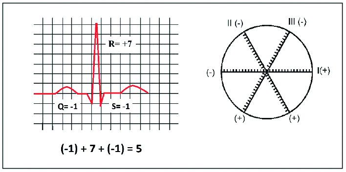


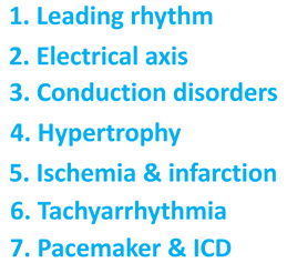


According to the expert opinion of the Polish Cardiac Society, the interpretation and report of an electrocardiogram (ECG) consists of 10 steps [1-2]. For the sake of simplicity, it is possible to simplify these rules to 7 steps. The ECG description should begin with the assessment of the baseline rhythm or rhythms (step 1). The electric axis of the heart should be analyzed in step 2. The next step (step 3) is the analysis of all supraventricular and ventricular conduction disorders, without which you cannot evaluate other pathologies in the ECG (ventricular hypertrophy, acute coronarysyndromes). Analysis of conduction disorders is best done step-by-step, starting from the highest “floor”(sino-atrial), then descending down the heart, to the atrio-ventricular and intraventricular "floors". In the next step, (step 4), the structure of the heart chambers should be assessed in terms of enlargement and hypertrophy. Step 5 analyzes all that is associated with ischemic heart disease, myocardial infarction and previous coronary events. This step also describes the morphology (shape) of ventricular complexes for pathological Q-waves, QS complexes, and R-wave changes. We then analyze the ST segment, T-wave and QTc interval associated with acute coronary syndromes. Step 6 describes tachyarrhythmias. The final step (step 7) is to describe the pacemaker and implantable cardioverter-defibrillator function in terms of effective pacing and possible malfunctions of sensing (Figure 1).
Figure 1. The 7 steps of ECG interpretation
Step 1 – Assessment of the leading rhythm or rhythms
When using the ECG in differential diagnosis of heart disorders, the first and fundamental step is to correctly assess the heart’s rhythm. This should be done in three small steps (Figure 2).
Figure 2. Assessment of the leading rhythm or rhythms
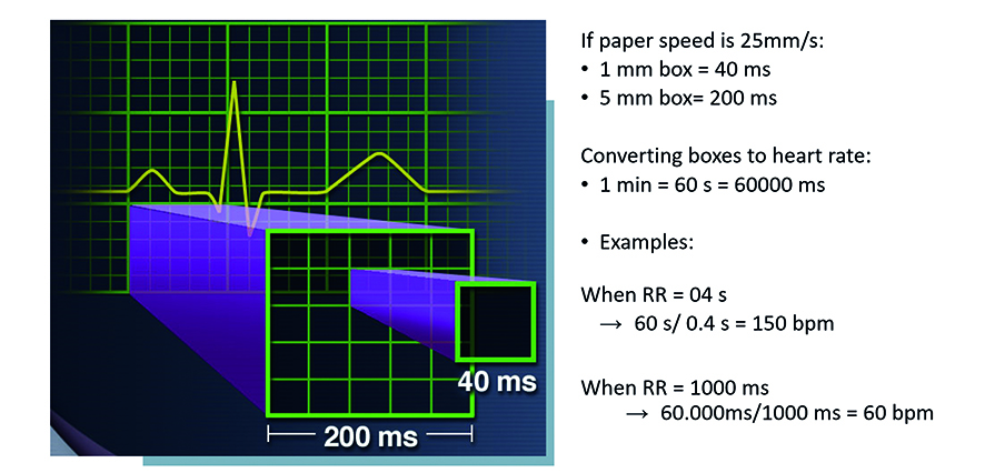
First, assess the rate of the rhythm. Normal heart rate (normocardia) is defined as 60-100 beats per minute. A slow heart rate (bradycardia) is < 60 beats per minute (bpm). Whereas an accelerated heart rate (tachycardia) is > 100 bpm. It is fundamental to assess the heartrate. All of the ECG tracings shown in this article are recorded at paper speed 25 mm/s with voltage 10 mm/mV. This means that each large square (5 mm) corresponds to 200 ms (0.20 s), while while 1 small square (1 mm) corresponds to 400 ms (0.04 s) and 1 m V = 10 small, 1 mm squares (Figure 3a). Thanks to this rhythm or rhythms standardization, each interval, segment and wave can be assessed in terms of duration in time.
Figure 3a. Assessing the rate of the leading rhythm
Source: Pacemaker Code and Rate and Interval Conversion pocket reference card (UC198801622m EN)
A simple way to approximate the heart rate on a 25 mm/s ECG tracing is the co-called “300 Rule.” According to this rule, divide 300 by the number of large squares between the peaks of two R waves (RR , a quick refresher about ECG waves is in Figure 3b). In the previous example, the RR interval was 400 ms (0,4 s), which corresponds to 2 large squares. Therefore, 300 divided by 2 equals 150, a heart rate of 150 bpm. At the paper speed of 50 mm/s, all the above-mentioned parameters need to be doubled, thus making it “The 600 Rule.”
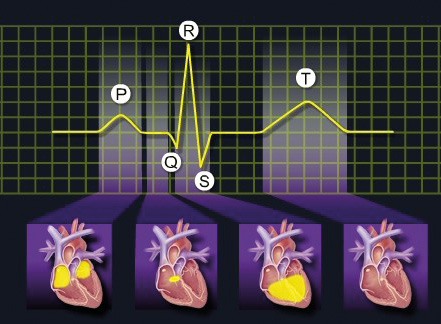
Figure 3b. Cardiac muscle activity and the corresponding ECG waves
Source: Pacemaker Code and Rate and Interval Conversion pocket reference card (UC198801622m EN)
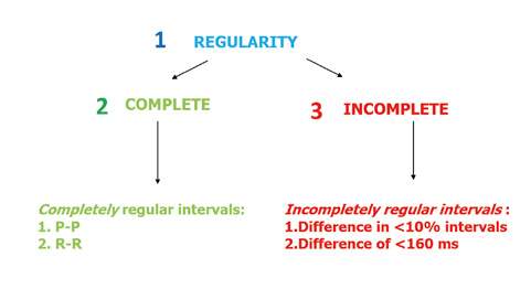
The second small step is to assess whether the rhythm is regular or irregular (Figures 4 and 5). Differentiating between the various types of regularity is not always simple because the human heart and its activity is influenced by the autonomic nervous system. Therefore we can recognize rhythms that are completely regular and incompletely regular.
Figure 4. Assessing the regularity of the leading rhythm
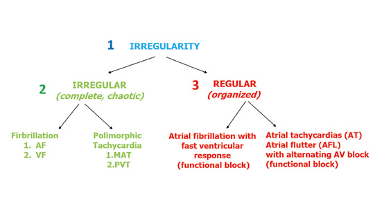
Figure 5. Assessing the irregularity of the leading rhythm
A completely regular rhythm is such when using a compass or ECG ruler you determine that the intervals between the P or R waves are equal to in every beat. Sometimes a slight irregularity in the rhythm is noted (Figure 4). In such situation, an incompletely regular rhythm is defined if the intervals between the P waves and QRS complexes (PQ intervals) are different from each other in < 10% of the preceding intervals or by 160 ms of the preceding intervals.
The assessment of irregular rhythms is much simpler. When documenting the rhythm as irregular, you need to note whether it is completely chaotic or somewhat organized. There are no precise criteria to differentiate those two types of irregular rhythms. A chaotic irregular rhythm cannot be organized in any way, e.g. atrial fibrillation. Whereas a more regular irregularity is best seen in tachycardias with a functional alternating A-V block (Figure 5).
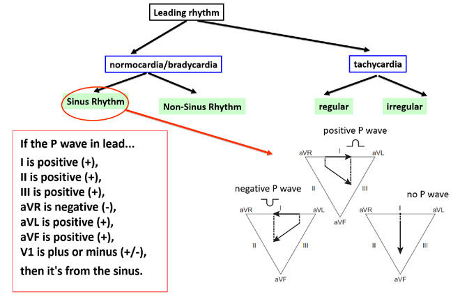
The third and final step of rhythm assessment is to determine its source (is this a sinus or non-sinus (atrial or nodal) rhythm?). Figure 6 shows the above-described steps in assessment of the leading rhythm in the atria.
Figure 6. Assessing the P wave. (+) = upward deflection (above the isoelectric line) (-) = downward deflection (below the isoelectric line)
The key is to assess the morphology (shape) of the main wave of atrial depolarization, either the P wave (sinus rhythm) or a P’ wave (non-sinus atrial rhythm). If the particular rhythm is of sinus origin, then the impulse should propagate (spread) from the top to bottom of the atria and at the same time from the left to right side. This results in the normal correct polarization of P wave deflections we see in particular leads. The inferior leads II, III and aVF best show the top-to-bottom direction of the propagation of depolarization. In case of a sinus rhythm, the P waves in those leads should be all positive (+). In order to assess whether the sinus rhythm propagates from the right atrium to the left atrium, pay attention to leads aVR and aVL. A normal atrial depolarization wave (in other words an impulse from the sino-atrial node) must move away from the aVR lead (negative (-) P wave) and towards the aVL lead (positive (+) P wave). Limb lead I can be helpful in assessing the source of the rhythm (Figure 6).
If after analyzing the above-mentioned leads you are still not sure of the rhythm, then it is worth to look at one of the precordial leads (e.g. V1). The V1 lead is positioned above the right ventricle but in the transverse plane, therefore it does not show atrial activation as clearly as the previously mentioned leads. In lead V1 an impulse propagating from the right atrium will have a positive-negative deflection (±), whereas an impulse propagating from the left atrium will be shown as a positive P wave (+).
It is worth adding that the aVR and aVL leads can provide more details, such as propagation of impulses from the lateral walls of the atria, the common atrial septum and from the superior or inferior parts of the atria. In the first situation the P wave deflections are in opposite directions, while in the second situation they point to the same direction. If the P wave is negative (-) in the aVR lead and positive (+) in aVL → the impulse is propagating from the lateral wall of the right atrium. If the P wave is positive (+) in the aVR lead and negative (-) in aVL → the impulse is propagating from the lateral wall of the left atrium. Additionally, if the P waves are negative (-) in both the aVR and aVL leads → the impulse is propagating from the superior part of the interatrial septum. If the P waves are positive (+) in both the aVR lead and aVR leads → the impulse is propagating from the inferior part of the interatrial septum. The limb lead I shows whether the impulse propagated from the right atrium (positive (+) P wave) or the left atrium (negative (-) P wave). All of the above details are summarized in Figure 6.
Step 2 – Assessment of the electric axis of the heart
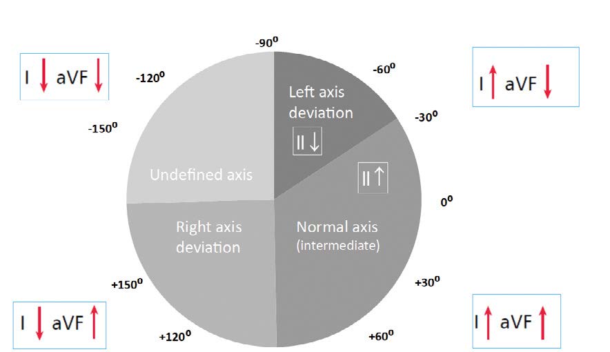
It is important to remember that electric axis should not be assessed in case of tachycardia or lack of intrinsic QRS complexes (e.g. paced rhythm). It is best to assess the electric axis using limb leads I and aVF. Lead II is useful in assessing a left axis deviation. The following types of electric axis can be seen in ECGs: normal axis (sometimes referred to as intermediate axis) (-30° to +90°), right axis deviation (+90° to +180°), left axis deviation (-30° to -90°), indeterminate axis (sometimes referred to as Northwest axis) (-90° to -180°) (Figure 7).
Figure 7. Assessing the electrical axis of the heart
As mentioned earlier, the latest guidelines state that the electric axis of QRS complexes should be assessed based on the inferior lead aVF (instead of lead III as was taught in the past [2]). In addition, the old term “physiological left axis deviation” is no longer in use because left axis deviation is always pathological. Thus normal axis is now referred to as intermediate and defined by positive QRS deflections in I and aVF (right half of the wheel). If the QRS complex is positive in lead I but negative in aVF, then assess lead II. If in lead II the QRS net is positive, then the axis is still intermediate (normal), whereas if negative then the ECG shows a left axis deviation. If the net QRS in lead I is 0, then it means that the electrical axis in that lead is perpendicular, either +90° or -90°. Therefore, the net QRS in aVF, II, III will help decide if the electrical axis of the heart is normal (+90°) or left (-90°).
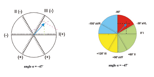
Precise measurement of the electric axis of the heart using the Cabrera’s wheel with the Einthoven’s triangle is shown in Figures 8 and 9, whereas Figure 10 shows the main causes of its deviation.
Figure 8. Assessing the electrical axis of the heart – calculating the QRS net
Adapted from www.registerednursern.com
Figure 9. Assessing the electrical axis of the heart – calculating the QRS net
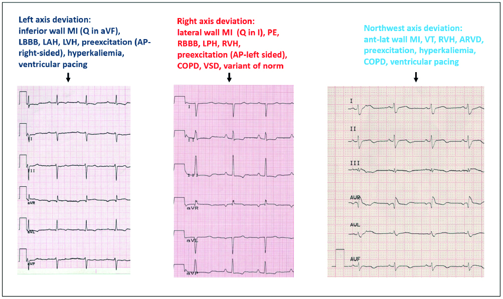
Figure 10. The many etiologies of heart axis deviation
AP – accessory pathway, ARVD – arrhythmogenic right ventricular dysplasia, COPD chronic obstructive pulmonary disease, LAH – left anterior hemiblock, LBBB – left bundle branch block, LPH – left posterior hemiblock, LVH – left ventricular hypertrophy, MI –myocardial infarction, PE – pulmonary embolism, RBBB – right bundle branch block, RVH – right ventricular hypertrophy, VSD – ventricular septal defect, VT – ventricular tachycardia
Adapted from Baranowski, Warsztaty EKG
Step 3 – Assessment of conduction disorders
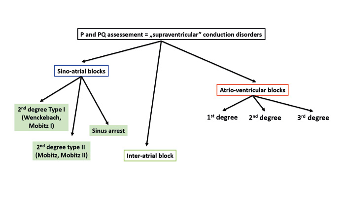
Step 3 is to assess conduction disorders. In the atria there can be sino-atrial (SA) conduction blocks or interatrial blocks. Sino-atrial blocks can be diagnosed after a sudden change in heart rhythm, most often a sudden bradycardia. In such cases you must pay attention which parts of the ECG tracing are missing or “dropped.”
A sino-atrial block causes a missing P wave and also the following QRS complex. Whereas if only the QRS complex is missing, then it is an atrio-ventricular (AV) block.
As mentioned above, a sino-atrial (SA) block can be diagnosed only on a tracing that shows a change of rhythm from normal to sudden bradycardia (or vice-versa). On such ECG tracing there is an obvious difference between the sinus rhythm that often is twice as fast as the bradycardia.
SA blocks are not subdivided into 1st-3rd degree the way atrioventricular blocks are. The reason is that a 1st degree SA block is impossible to assess on a standard ECG and it appears very similar to respiratory sinus arrhythmia. Whereas a 3rd degree SA block is very difficult to differentiate from a pause due to sinus arrest.
The biggest challenge is to differentiate a 2nd degree SA block type I (Wenckebach) from type II (Mobitz). In type I the PP interval becomes shorter and shorter until it suddenly extends (pause). Whereas in type II there are intermittent missing P waves and such pauses are multiples of the PP interval (± 100ms). Finally, an ECG of a patient with sinus arrest shows a gradual prolongation of the PP interval followed by a sudden pause. The pause usually lasts > 2 seconds and on the tracing appears as 140% of the PP interval’s length (Figure 12a, 12b).
Figure 11. Assessment of conduction disorders
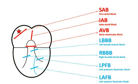
Figure 12a. Electrocardiographic features that differentiate sinoatrial blocks
Figure 12b. Conduction disorders depending on the location
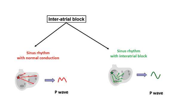
Interatrial (IA) blocks are disorders of conduction between the right and left atria. These blocks are recognizable by a changed shape of the P wave without changes in rhythm. One example can be an intermittent tall or deformed P wave imitating P pulmonale or P mitrale in a patient without valve disease. The main criterion is excess prolongation of a biphasic P wave (first phase positive, second phase negative) in inferior leads II, III and aVF. The reason why the P wave is biphasic is that the impulse traveling towards the AV node reaches the left atrium and stimulates it in the non-physiological direction from bottom to the top (Figure 13).
Figure 13. Conduction disorders: inter-atrial block
Blocks that involve the inferior part of atria, more specifically the atrioventriocular junction are referred to as atrioventriocular (AV) blocks (Figure 14). These are the most common blocks and are rather simple to recognize on a tracing. It is worth remembering that the physiological path of depolarization in the heart isas follows:
(1) SA node,
(2) working muscle of the atria,
(3) AV node,
(4) Bundle of His,
(5) Bundle branches,
(6) working muscle of the ventricles.
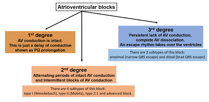
Figure 14. Conduction disorders: atrioventricular blocks
This physiological sequence is referred to as atrio-ventricular association and is seen on an ECG tracing as PQ interval (corresponds to AV conduction, as shown in Figure 14) of 120-200 ms (0,12-0,20 s). The first subtype is 1st degree AV block which is defined as prolonged duration of conduction through the AV junction. A good term for it is concealed block because it does not cause any clinical symptoms. On an ECG tracing it is recognized by PQ (or PR) interval prolonged > 200 ms consistently with each QRS (with intact atrio-ventricular association).
A 2nd degree AV block (also referred to as partial block) causes fewer impulses to be conducted to the ventricles (as the name suggests, some impulses are blocked at the AV junction). It causes conduction of every other (or less) impulses with normal duration. There are 4 subtypes of this block: type I (Wenckebach), type II (Mobitz), type 2:1 and advanced block.
In 2nd degree AV block type I (Wenckebach; in US and Canadian literature referred to as Mobitz I), there is a prolonged duration of AV conduction (gradual prolongation of the PQ/PR interval) to the point that the particular impulse is not conducted at all and there following P wave is not followed by a QRS complex (in clinical jargon this is a “dropped QRS”).
In 2nd degree AV block type II (Mobitz; in US and Canadian literature referred to as Mobitz II) the PQ (PR) interval is constant but some P waves are not conducted to the ventricles, thus missing QRS complexes are seen on the tracing. This block can have a regular time intervals, such as 3:2 (3 P waves for every 2 QRS complexes), 4:3 or 5:4.
The 2:1 AV block is somewhat between the Type I and Type II block. Currently this block is considered separate because its mechanism is between that of Type I (PQ prolongation leading to a blocked impulse) and Type II (blocked impulse without preceding PQ prolongation). If more than one QRS is blocked (e.g. 3:1, 4:1), then an advanced block is diagnosed.
3rd degree AV block is a complete block of all conduction between the atria and ventricles. It is a situation in which the atria have their own rhythm (e.g. from the SA node), while the ventricles rely on their own escape rhythm.
There are two types of 3rd degree AV blocks: proximal and distal. A proximal 3rd degree AV block is recognized by junctional (escape) beats with narrow QRS complexes and an escape rhythm of ~40‑50/min. Whereas in distal 3rd degree AV block the escape rhythm is generated by the Purkinje fibers which leads to wide QRS complexes at a slow rate of ~25-35/min. A distal 3rd degree AV block is usually seen in patients with MAS (Morgagni-Adams-Stokes) Syndrome (also referred to as cardiogenic syncope) which is a medical emergency and an absolute indication for immediate admission to the hospital. If the patient with MAS does not have a ventricular escape rhythm (only P waves are seen on the heart monitor or ECG tracing) → resuscitate immediately and call for help.
Figure 16. Ventricular (QRS) complex morphology in RBBB
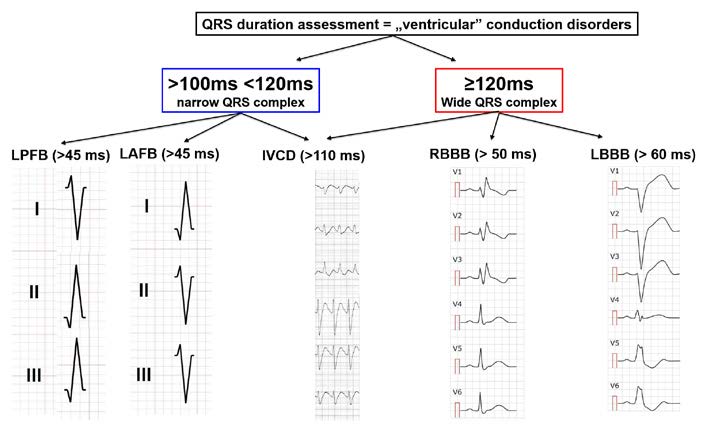
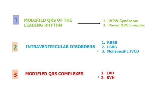
Figure 17. Conduction disorders: QRS assessment
Adapted from medrevise.co.uk, ems12lead.com
An intraventricular block is a delay of conduction in any part of the heart located inferiorly to the AV bundle (bundle of His) (Figure 15). Such block is usually caused by an interruption of conduction along the fibers of the respective branches of the AV bundle (right – RBBB and left – LBBB) or of the respective fascicles of the left bundle branch (anterior – LAFB or posterior – LPFB). To diagnose an intraventricular block, the ECG tracing must show wide QRS complexes (> 0.12 s) and a delayed intrinsicoid deflection in the blocked area. In this situation, part of the cardiac muscle is no longer stimulated, therefore the shape of the QRS complex is changed, which allows us to diagnose intraventricular blocks.
To diagnose right bundle branch block (RBBB) all of the following criteria must be met:
(1) wide S waves > 40 ms or S > R in leads I and V6,
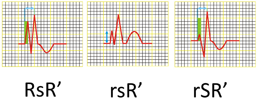
(2) QRS complex shaped as RsR’ or rSR’ or rsR’ in leads V1 and/or V2 (see Figure 16),
(3) wide QRS (> 0,12 s),
(4) delayed intrinsicoid deflection ≥ 50 ms in V1, and
(5) deflections of ST-T opposite of the QRS deflection in V1.
In RBBB, the early part of the QRS complex has a normal shape. Only after 40-60ms the QRS becomes deformed with a secondary R wave in the right ventricle leads and a deep S wave in the left ventricle leads. This is due to the pathological right deviation of the mean electrical vector of ventricular depolarization.
Thus, in RBBB the QRS complexes in leads V1 and V2 are tall double spikes and usually have an rsR' or rSR' configuration (Figure 6). Sometimes they only consist of a wide, double-spiked R wave or have a qR configuration. In leads I, II and the LV anterior leads the QRS complexes consist of a narrow R wave and a wide „showel-like” S wave. In cases of RBBB the electrical axis of the heart is usually normal and rarely deviated to the right or left. In case of an ECG tracing in which the QRS complexes have a shape that meets the criteria of RBBB but their width is > 0.10 s but < 0.12 s, you may only diagnose an incomplete RBBB.
To diagnose a complete left bundle branch block (LBBB) all of the following criteria must be met:
(1) wide, double-spiked R wave in leads V5, V6 and aVL,
(2) no Q wave in leads I and V6,
(3) wide QRS complex > 0,12 s,
(4) delayed intrinsicoid deflection ≥ 60 ms in leads V5 and V6 (optionally in I and/or aVL),
(5) ST-T level opposite to the QRS deflections in V5‑V6.
In sum, in leads V1-V2 QRS complexes are negative with short R waves or none at all (in such case that does not indicate necrosis of the myocardium) and deep S waves. In leads V5 and V6 the QRS complexes are positive, monophasic and with a double-spiked peak or ascending limb of the complex. Another sign of LBBB is the lack of „septal” Q wave in leads I, aVL, V5 and V6, corresponding to initial depolarization of the intraventricular septum from left to right. Whereas in the ECG of a patient with LBBB the presence of Q waves in the above-mentioned leads is pathological and suggests ischemia of the apex or the antero-lateral wall of the heart. Always remember that a new diagnosis of LBBB (the block not present in previous ECG tracings) and chest pain are highly suggestive of acute coronary syndrome and such patient requires consultation with the nearest cardiac catherization (invasive cardiology) laboratory.
Downsloping ST segment depression and negative T waves also fit in the picture of LBBB. Remember that a lack of this reciprocity does not mean a diagnosis of anterior or lateral wall ischemia. Negative T waves in the precordial leads should be interpreted with caution as they can be a sign of myocardial ischemia or non-specific changes due to cellular memory of an abnormal depolarization pathway. In LBBB the electrical axis of the heart is usually normal (intermediate axis).
In left anterior fascicular block (LAFB; sometimes referred to as Left Anterior Hemiblock – LAH) all of the criteria below must be met:
(1) left axis deviation (+45⁰ to +90⁰),
(2) qR configuration of the QRS complex in lead aVL,
(3) a wide R wave (time to peak of the R wave > 45 ms in lead aVL),
(4) narrow QRS < 120 ms.
Similarly, in order to recognize a left posterior fascicular block (LPFB), all of the following criteria must be met:
(1) right axis deviation (+90⁰ to +180⁰),
(2) qR complexes in leads III and aVF,
(3) rS complexes in leads I and aVL,
(4) time to the peak of the R wave >45 ms in leadaVF,
(5) QRS complex <120 ms and
(6) no signs of right bentricular hypertrophy (RVH).
In LPFB the q wave in leads III and aVF does not need to meet any criteria of width or amplitude. In case the Q waves meet the criteria of pathological Q wave, then you must diagnose ACS and LPFB. If the QRS is wide, then it is not possible to recognize LPFB (except in patients with coexisting RBBB).
Step 4 – Assessment of the hypertrophy of cardiac chambers
To assess left ventricular hypertrophy (LVH) you need to use criteria based on voltage. The two most commonly used are: Cornell Criteria (height of S wave in V3 + height of R wave in aVL >28 mm (♂), > 20 mm (♀) and the Sokolov-Lyon Index (S in V1 + R in V5/V6 > 35 mm (> 40 years old), > 40 mm (30-40 years old), > 60 mm (16-30 years old). There are also other criteria such as R-V5 > 26 mm, R-V6 > 20 mm, the largest R + S > 45 mm in any precordial lead or S-II + R-I > 26 mm in limb leads, R-aVL > 12 mm (except for LAH), R-I > 14 mm, SaVR > 15 mm and delayed intrinsicoid deflection > 0,05 (V5, V6) with downsloping ST segment depression and negative T wave.
For the right ventricular hypertrophy (RVH) the criteria are: dominant R in V1 ≥ 7 mm, sum R in V1 + S in V5 or V6 > 10,5 mm, R/S ratio in V1 > 1or R/S in V5/V6 ≤ 1, rSR’ in V1 with R’ > 10 mm, qR complex in V1 and delayed intrinsicoid deflection > 0,035 s (in V1-V2) but < 0,05 s, deep S in V5-V6 and downsloping ST segment depression, negative T wave, asymmetric, negative-positive, and in V1, V2 asymmetric, negattive-positive. The simplified criteria of hypertrophy in ECG are shown in Figure 18.
Figure 18. Assessment of cardiac hypertrophy
Atria should also be assessed for hypertrophy (enlargement). Right atrial enlargement (RAE) is recognized by a specific shape of the P wave, known as P-pulmonale (> 2,5 mm tall P wave in at least one limb lead and a > 1,5 mm tall P wave in V1 or V2. Whereas left atrial enlargement (LAE) produces P-mitrale (P wave that is > 120 ms long, time between its two peaks (or humps) ≥ 40 ms or a positive-negative or negative P wave in V1 (negative phase at least 0,04 s and 1 mm deep). Remember that the patient can have hypertrophy/enlargement of both chambers (i.e. both atria or both ventricles). In order to diagnose hypertrophy of both ventricles, at least one RVH and at least one LVH criteria must be met.
Different criteria exist for hypertrophy of both ventricles (LVH+RVH): deep S waves in V5 or V6 or right axis deviation and tall double-spiked QRS complexes in several leads. Such biventricular hypertrophy usually presents with tall biphasic RS complexes in precordial leads V2, V3, V4 (Katz-Wachtel phenomenon).
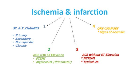
Step 5 – Assessment of ischemic changes and infaction
The next step is the assessment of the ST segment (1), T wave (2) and Q waves (3) in terms of acute coronary syndromes (unstable angina, STEMI, NSTEMI) and necrosis in the past (Figure 19). The key guidelines are described in the Fourth Universal Definition of Myocardial Infarction [3]. An ST segment elevation that is new and extended in duration (e.g. > 20 minutes), especially with reciprocal ST depression in other leads is highly pathognomonic for acute coronary syndrome (ACS). Such ECG findings usually correspond to acute occlusion of a coronary artery and causes myocardial ischemia with necrosis. Besides the above-mentioned ST changes, myocardial ischemia or acute infarction might also cause PR segment and/or QRS changes (Figures 20 and 21).
Figure 19. Assessment of ischemic changes and infarction
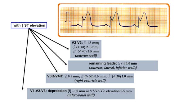
Figure 20. Ischemic changes and infarction: Criteria for ischemic
changes and infarction with ST segment elevation
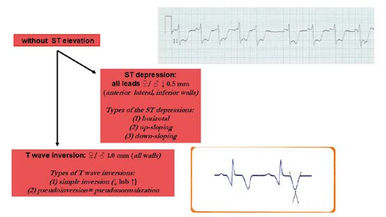
Figure 21. Criteria for ischemic changes and infarction without ST elevation
The earliest ECG signs of myocardial ischemia are T wave and ST segment changes. Tall, positive and symmetric T waves in at least 2 contiguous leads (referring to the same wall of the heart, see below) are an early sign of ACS and might appear sooner than ST elevation. Intermittent Q waves might be seen in ECG of a patient during acute ischemia and (rarely) during acute infarction after successful reperfusion.
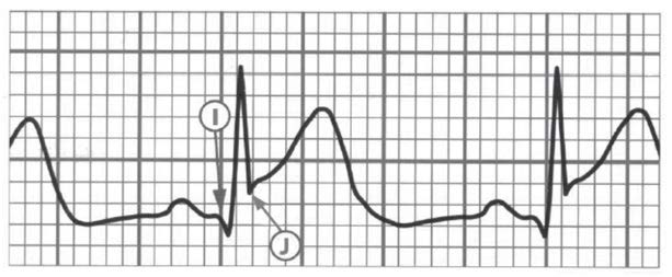
Another important element to pay attention to is the J point which links the QRS complex with the ST segment (Figures 21, 22 and 23). The J point is used to assess the amount of ST segment elevation or depression in cardiac ischemia regards the TP segment (isoelectric interval). Sometimes during the tachycardia this determination is difficult. The Q wave onset (I-point) is recommended as the reference point for J-point determination (Figure 22). Except for V2 and V3, to make the diagnosis, the ECG must show a new (or presumably new) ST segment elevation by at least 0,1 mV (1 mm). Remember that healthy men < 40 years of age can have a physiological J point elevation of up to 0,25 mV in lead V2 or V3, decreasing with age. Whereas healthy women can have up to 0,15 mV J point elevation (Figure 20). Just as ST segment changes, the J point elevations need to be shown in contiguous leads: anterior leads (V1–V6), inferior leads (II, III, aVF) and lateral leads (I, aVL). Additional leads such as V3R and V4R correspond to right ventricle, whereas leads V7-V9 correspond to the posterior (inferobasal) wall (Figure 20).
It is important to remember that acute myocardial ischemia rarely causes ST segment changes that meet the criteria in just one lead. Furthermore, ST segment and T wave changes that do not meet the criteria do not exclude ACS or an evolving myocardial infarction. During an episode of acute chest pain, a pseudonormalization of T waves which were previously negative might also indicate acute myocardial ischemia (Figure 22).
Figure 22. The I-point (onset of Q wave as a reference point) and the J-point (the junction of the S wave and the ST segment)
Because many conditions cause ST segment and T wave changes, the differential diagnosis of primary ST-T changes in an ECG of a patient with chest in pain must always include:
(1) pulmonary embolism,
(2) electrolyte imbalance,
(3) hypothermia,
(4) pericarditis,
(5) myocarditis,
(6) stroke.
Therefore, when interpreting & describing the ECG you must decide if the ST-T changes are primary (typical of myocardial ischemia), secondary (due to non-ACS such as depolarization wave disturbances e.g. pre-excitation syndromes), non-specific (do not meet the criteria of primary nor secondary) or perhaps chronic (due to past ACS) (Figure 19, 23).
Figure 23. Secondary changes of the ST Segment and T-wave
In patients with LBBB it is more difficult to recognize the ECG changes due to acute ischemia. In such situations it is helpful to look for ST elevations of > 1 mm in the same direction as QRS complexes. If the QRS complexes are negative (downwards), then the ST elevations must meet the criterion of > 5 mm at the J point. Remember that in case of LBBB the contiguous leads criterion no longer applies, therefore an ST segment change in just one lead is sufficient. Whereas ST depressions must be > 1mm deep at the J point. In patients with RBBB there are often ST-T changes (e.g. ST elevations and pathological Q waves) in leads V1-V3, such as ST elevations and pathological Q waves.
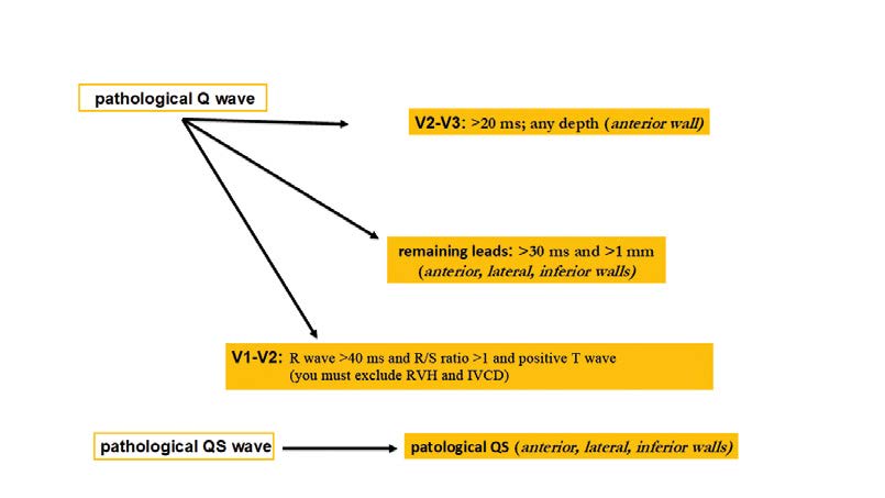
Regardless of clinical symptoms, Q waves or QS complexes without the presence of factors that alter the QRS shape are pathognomonic for myocardial necrosis in patients with ischemic heart disease. The ECG changes indicating a past ACS are most specific when Q waves appear in several leads or groups of leads. If the Q waves coexist with ST or T changes in the same leads, then the likelihood of past ACS is greater, but not certain. This applies to Q waves that are > 0,02 s and < 0,03 s and < 0,1 mV deep. Such Q waves usually indicate a past MI if coexisting with negative T waves in the same group of leads. That is why the ECG is not the tool to assess the time elapsed since a coronary event (Figure 24).
Figure 24. Ischemic changes and infarction: pathological Q waves and QS complexes
Although the ECG is poor at estimating the time of ischemia, we cannot treat every ECG tracing with signs of myocardial ischemia as evidence of an ACS. ST segment assessment has several pitfalls that lead to wrong diagnosis. The most common of which is a wide QRS due to intraventricular blocks (because it causes secondary ST changes) or QT prolongation (because the shape of T wave is changed). Please remember that ECG is only one of several tests that suggests the presence (or absence) of certain pathologies and the final clinical diagnosis is the sum of many other pieces of information.
Step 6 – Assessment of arrhythmias
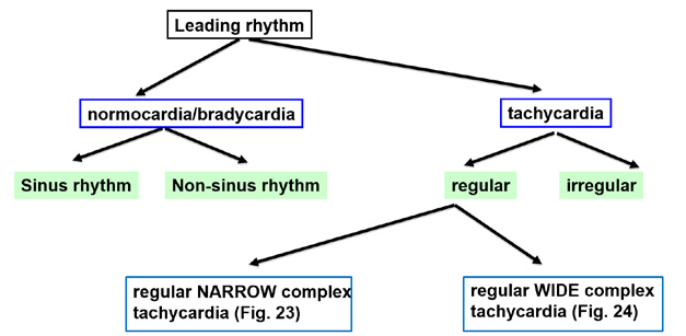
In case of tachycardia (> 100 bpm), it is fundamental to distinguish regular from irregular rhythms. The regular algorithm further differentiates regular tachycardias into narrow complex (QRS < 120 ms; determines precise origin of the tachycardia) and wide (broad) complex (QRS > 120 ms, determines ventricular or non-ventricular origin) (Figure 25).
Figure 25. Assessment of arrhythmias
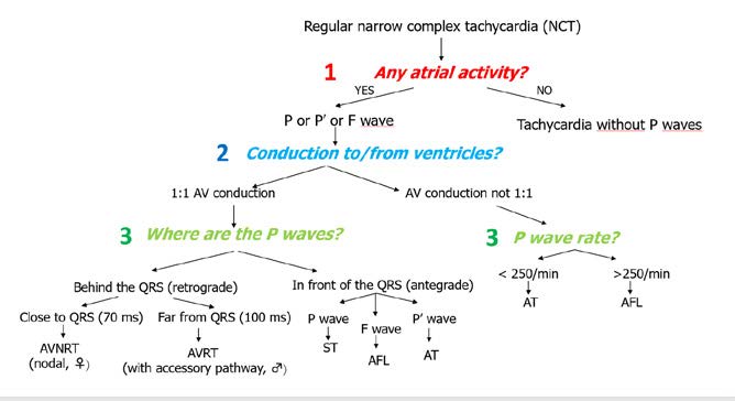
When analyzing regular tachycardias, it is fundamental to carefully look for waves that confirm the function of particular cardiac chambers. This is much easier to do in case of narrow complex tachycardias. The algorithm shown in Figure 26 allows diagnosing the particular type of tachycardia. However the first and key step is to make sure that the tachycardia is indeed regular.
Figure 26. Arrhythmias: regular narrow complex tachycardia
The next step is to focus on atrial function and find P, P’ or F waves. Afterwards, the next step is to the AV conduction and the algorithm splits into 1:1 and non 1:1 conduction.
The most common examples of non-1:1 conduction are atrial tachycardia (AT) or atrial flutter (AFL). AT is < 250 bpm and characteristically presents with P’ waves with a segment of isoelectric line. Whereas AFL is faster(atria contract at 250-300 bpm), with 2:1 conduction and instead of the isoelectric line there is a sawtooth pattern of F waves.
In case of 1:1 conduction, the key question is: where are the P waves in relation to the QRS complexes during the tachycardia – in front of or behind the QRS complexes? To answer it, measure from the start of the R wave to the start of the P’ wave. If P’R > RP’ then the P’ wave is behind the QRS complex, whereas if P’R <RP’ then it is in front of the QRS.
If the PI wave is behind the QRS complex then it means that the atria are stimulated after the ventricles are stimulated, which means there is a reentry pathway and only two arrhythmias are possible: AVNRT or AVRT. The first spins in the AV node, while the second spins between the atria and ventricles via additional pathway (Wolf-Parkinson-White syndrome). In order to properly differentiate them:
RP' distance < 70 ms → AVNRT
or > 70 ms → AVRT
If the AV conduction is 1:1 and the P waves are in front of the QRS complexes, then the depolarization isdownward (antegrade activation, not reentry). In such case, analyzing the P wave is sufficient to recognize the type of tachycardia. If the P wave meets the criteria of sinus wave (see Figure 6), then the tachycardia is sinus in origin as well (sinus tachycardia, ST). If the P wave does not meet the sinus criteria, then the rhythm is atrial tachycardia (AT). Whereas if the wave has a “sawtooth” pattern, then it is an F wave of atrial flutter (AFL) with 1:1 conduction.
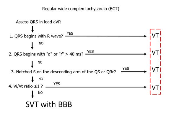
One of the simplest algorithms for differentiating wide complex tachycardias (WCT) is the aVR algorithm, also known as the regular wide complex tachycardia algorithm (Figure 27). It was designed by a team of mostly Hungarian cardiologists, therefore it is is often referred to as the Vereckei algorithm, after its first author. The underlying principle of this algorithm is to assess the speed of ventricular conduction shown in lead aVR [4]. Specifically, the key is to assess the rate of the first and last 40 ms of the QRS complex in a wide complex tachycardia. If the WCT is caused by a supraventricular tachycardia (SVT), then the initial activation of the septum should be fast and slows down at the end of activation. Whereas during a WCT caused by ventricular tachycardia (VT) the situation is opposite: the initial activation is initially slower than in the final phase.
Figure 27. Arrhythmias: regular wide complex tachycardia
Assessment of QRS complex morphology (shape) is focused on finding the dominant R wave in the aVR lead – this is critical for diagnosing VT. In addition, the R wave needs to be the beginning of the QRS complex (so-called initial R wave). If such initial R wave is present in the QRS complex, then the patient has VT and requires EKG monitoring and treatment because of high risk of becoming hemodynamically unstable and requiring resuscitation. If not, then check if a q or r wave > 40ms is present. If yes, then the patient also has VT and requires treatment. Finally, if check if a notched S wave is present on the descending arm of the QS or QSr complex in lead aVR. If yes, then once again the patient has VT and requires treatment. In summary, presence of a monophasic R wave or an Rs complex (which occur in ~40% of VT) in the ECG is sufficient to diagnose VT and finish differential diagnosis.
If none of the above criteria are met, the next step is to assess the Vi/Vt (ventricle initial/ventricle terminal) in lead aVR. The Vi/Vt criterion is also based on assessing the rate of increase of the first and last 40 ms of the QRS complex. In the 40 ms segment you count how many small (1 mm) boxes-long is the QRS complex. The first 40 ms is the Vi (initial part of ventricular complex), while Vt is the final 40ms is the terminal part. A Vi/Vt ≤ l indicates VT, whereas Vi/Vt >1 indicates SVT with BBB.
Let’s not forget that tachycardias can also present as irregular rhythms and therefore require different criteria of assessment (Figures 28 and 29). The most common irregular tachycardia is atrial fibrillation (AF). This is also the most common of all arrhythmias and it can be easily recognized on the ECG by the lack of P wave (due to irregular electrical/mechanical activity of the atria). Instead of P waves, AF presents withirregular and polymorphic fibrillation waves (f waves, usually > 300-350/min, best seen in V1 and V2) and usually a completely irregular rate of QRS complexes. However, in some patients AF presents with a regular ventricular response (QRS complexes appear regularly on the ECG) and this situation usually occurs in:
(1) the presence of an arrhythmia other than AF, e.g. atrial flutter (AFL),
(2) the presence of a complete III⁰ block with an escape rhythm from the AV junction (narrow complex) or from the ventricles (wide complex),
(3) the presence of nonparoxysmal junctional tachycardia (NPJT) or ventricular tachycardia (VT) or accelerated idioventricular rhythm (AIVR),
(4) constant ventricular pacing in VVI mode or in case the device switches to the VVI mode (DDD → VVI).
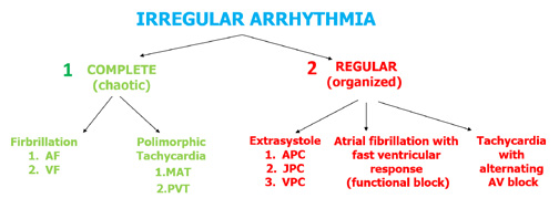
Figure 28. Assessment of irregular arrhythmias
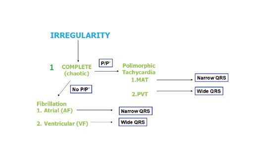
Figure 29. Arrhythmias: assessment of complete irregularity
Another example of a fast and irregular rhythm is multifocal atrial tachycardia (MAT) which presents with polymorphic P’ waves with various conduction to the ventricles (Figure 28). If this irregular rhythm is organized, then most often it is caused by additional, premature atrial, junctional or ventricular contractions (APC, JPC and VPC, respectively). A detailed algorithm for assessing irregular rhythms is shown in Figure 30.
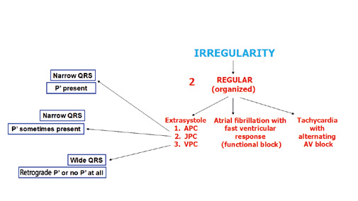
Figure 30. Arrhythmias: assessment of organized irregularity
Another irregular wide complex tachycardia is a polymorphic ventricular tachycardia (PVT). In such arrhythmia the wide QRS complexes constantly (from beat to beat) change their morphology (hence the name “polymorphic”). An example is PVT is torsade de pointes (TdP), an arrhythmia in which the QRS complexes change their amplitudes and „twist” 180⁰ across the isoelectric line every 10-15 beats. In contrast to a bidirectional tachycardia, this change of morphology occrurs smoohtly. Torsades de pointes is a life-threatening arrhythmia and such patient requires an immediate intravenous bolus of magnesium sulphate (2g administered over 10 minutes). If the patient has no pulse, defibrillate immediately and resuscitate according to your country's current resuscitation guidelines [5].
The most common regular (organized) arrhythmias (allorytmia rhythmica) are additional atrial or ventricular contractions (Figure 30). Atrial premature contractions (APC) are one of the most common causes of irregular heart rate. They can originate anywhere in the SA node, the atria or the AV junction. They present with characteristic P’ waves and narrow QRS complexes. In case of APC originating in the AV junction, the P’ waves appear as reentry waves (negative in II, III i aVF) or do not appear at all (usually hidden inside the QRS complex).
Premature ventricular contractions (PVC, also referred to as extrasystoles) are single additional impulses from the ventricular muscle tissue. Usually they appear as a premature and abnormally wide QRS complexes. Such 1:1 frequency is decribed as bigeminy, whereas a 1 PVC for every 2 conducted QRS complexes is described as trigeminy. After the PVC there might be a compensatory or non-compensatory pause, whose symptoms are completely opposite. Patients experience a compensatory pause as a sudden but short-lasting cardiac arrest after which the heart rate returns to normal. Whereas a non-compensatory pause does not cause the patients any symptoms despite the fact that their heart rate is disturbed. There are also interpolated VPCs, which essentially „double” the heart rate, while VPC with pauses cuase a „double” slowing down of the heart rate, a socalled pseudobradycardia.
Step 7 – Electrical pacing of the heart (pacemaker)
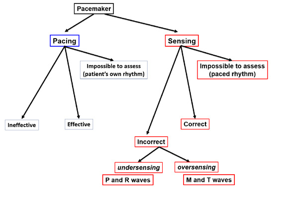
The final step is to assess the function of the implantable pacemaker or cardioverter-defibrillator. It is fundamental to determine if the device is effectively stimulating the heart and what type of disturbance of sensing is visible in the ECG (Figure 31).
Figure 31. Assessment of electrical pacing of the heart
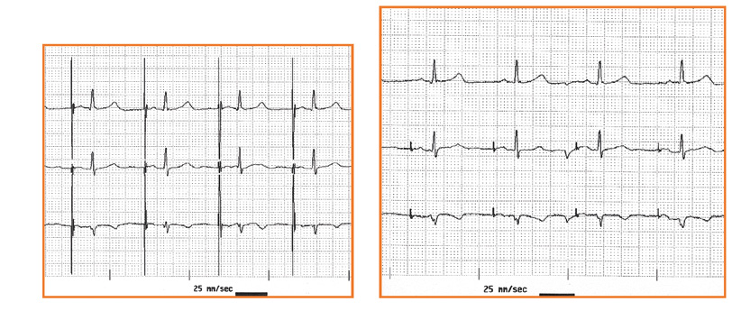
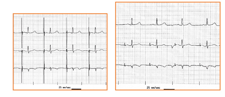
Effective pacing can be recognized on the ECG when the delivered „peak” is directly (the several milisecond-long delay is impossible to observe on a standard ECG tracing) followed by a wave from the stimulated chamber: a P wave (if atria are stimulated) or an R wave (in case of ventricular stimulation, see Figure 32). An exception to this rule are patients with a significant heart defect or hypertrophy withcoexisting fibrosis, because that delay might consistently last several dozen miliseconds. Whereas if the interval between the delivered peak and the chamber’s response is different from beat to beat, then it is highly likely that the device is not stimulating effectively.
Figure 32 a,b. Assesment of the type of pacing: unipolar vs bipolar
The definition of ineffective stimulation (pacing) is lack of visible QRS complex in < than 40 ms since the stimulating impulse. Note: it can be difficult to identify the delivered impulse in ECGs of patients with bipolar devices or atrial pacing. Furthermore, assessment of pacing effectiveness might be difficultwhen the shapes of the paced QRS and intrinsic (patient’s own) QRS complexes is similar. That is why it is helpful to analyze and compare the QRS complexes in all the available leads of the ECG. Remember that a lack of visible atrial or ventricularresponse to pacing might be due to the impulse being delivered exactly during the chamber’s refractory period, therefore you should not describe this situation as ineffective pacing.
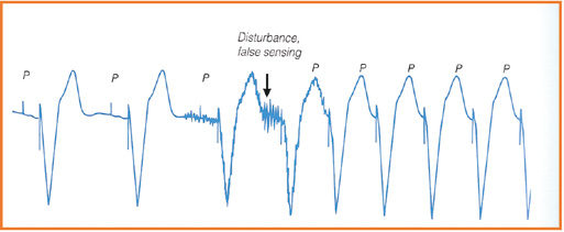
Besides pacing effectively, implanted devices must correctly receive and respond (referred to as sensing) to the heart’s intrinsic impulses. An implanted device might be functioning properly (correct sensing), or not sensitive enough to intrinsic impulses (undersensing) or be too sensitive to intrinsic impulses (oversensing). Undersensing usually involves intrinsic impulses form the myocardium: the atrial P wave and the ventricular R wave. Whereas oversensing tends to involve electrical waves from outside of the heart: skeletal muscle waves (M waves) and the repolarization wave (T wave, see Figure 33).
Oversensing M
Undersensing P
Figure 33. Failure of the sensing: oversensing vs undersensing
Figure 34. Evaluation of the implantable cardioverter-defibrillator (ICD) function
It is more difficult to assess an implantable cardioverter- defibrillator (ICD) than a pacemamker. It is most important to assess the effectiveness of defibrillation during an adequate intervention (discharge). Any malfunctions of defibrillation must be immediately repaired. In contrast, an inadeuate ICD discharge usually occurs during an episode of SVT (e.g. AF, AFL or AT). Although an inadequate discharge is very painful (20J of energy while being fully conscious), such situation is less dangerous for the patient but the device needs to be adusted by a cardiologist.
Acknowledgements
The author would like to thank Janusz Springer MD for the English translation and valuable input on the first draft of this paper.
References
| 1. |
Baranowski R, Wojciechowski D, Kozłowski D, Kukla P, Kurpesa M, Lelakowski J, et al. Electrocardiographic criteria fordiagnosis of the heart chamber enlargement, necrosis and repolarisation abnormalities including acute coronary syndromes. Experts’ group statement of the Working Group on Noninvasive Electrocardiology and Telemedicine of PolishCardiac Society. Kardiol Pol. 2016;74(8):812–819.
|
| 2. |
Baranowski R, Wojciechowski D, Kozłowski D, Kukla P, Kurpesa M, Lelakowski J, et al. Compendium for performing anddescribing the resting electrocardiogram. Diagnostic criteria describe rhythm, electrical axis of the heart, QRS voltage, automaticity and conduction disorders. Experts’ group statement of the Working Group on Noninvasive Electrocardiology and Telemedicine of Polish Cardiac Society. Kardiol Pol. 2016;74(5):493–500.
|
| 3. |
Thygesen K, Alpert JS, Jaffe AS, Chaitman BR, Bax JJ, Morrow DA, et al. Fourth universal definition of myocardial infarction (2018). Journal of the American College of Cardiology. 2018; 72(18), 2231-2264.
|
| 4. |
Vereckei A, Duray G, Szénási G, Altemose GT, Miller JM. Application of a new algorithm in the differential diagnosis ofwide QRS complex tachycardia. Eur Heart J. 2007;28(5):589–600.
|
| 5. |
Soar J, Nolan JP, Böttiger BW, Perkins GD, Lott C, Carli P, et al. European resuscitation council guidelines for resuscitation 2015: section 3. Adult advanced life support. Resuscitation, 2015; 95, 100-147.
|
